*Corresponding author.
Nonparametric inference on structural breaks
Miguel A. Delgado
!
, Javier Hidalgo
",
*
!Departamento di Estadistica y Econometria, Universidad Carlos III, cl Madrid 126-128, Getafe, 8403 Madrid, Spain
"Department of Economics, TGO London School of Economics and Political Science, Houghton Street, London WC2A2AE, UK
Received 1 January 1998; received in revised form 1 April 1999
Abstract
This paper proposes estimators of location and size of structural breaks in a, possibly dynamic, nonparametric regression model. The structural breaks can be located at given periods of time and/or they can be explained by the values taken by some regressor, as in threshold models. No previous knowledge of the underlying regression function is required. The paper also studies the case in which several regressors explain the breaks. We derive the rate of convergence and provide Central Limit Theorems for the es-timators of the location(s) and size(s). A Monte Carlo experiment illustrates the perfor-mance of our estimators in small samples. ( 2000 Published by Elsevier Science S.A. All rights reserved.
JEL classixcation: C14; C32
Keywords: Nonparametric regression; Dynamic models; Structural breaks; One-sided kernels
1. Introduction
This paper proposes estimators of the location(s) and size(s) of jump(s) in a, possibly dynamic, nonparametric multiple regression model where the jumps
are located at given periods of time and/or are explained by the values of some
regressors, as in threshold models. Regressors can be stochastic and/or"xed.
One of the main features of our estimators is that their asymptotic distribution is normal, in contrast to rival parametric ones, which are, in general, not distribu-tion free.
There is a vast literature on testing for the presence of a structural break when the possible timing of the break is unknown. See for instance, Quandt (1960), Hinkley (1969, 1970), Brown et al. (1975), Hawkins (1977), Worsley (1979), Kim and Siegmund (1989), Andrews (1993) and Andrews and Ploberger (1994). When a break exists, there is also some work on the estimation of the location of the break point, e.g. Feder (1975), Yao (1987), Eubank and Speckman (1994) and Bai (1994). The latter are typically based on a quadratic loss function, although robust estimators have been considered by Bai (1995), Antoch and Huskova (1997) and Fiteni (1998), among others. The previous work was done in a para-metric framework.
The parametric approach has two potential drawbacks. First, the asymptotic distribution of the estimators (location) typically depend on certain unknown features of the data generating process. Although this problem has been circum-vented by assuming that the size of the break shrinks to zero as the sample size increases, it appears that when the regressors are nonstationary (e.g. Bai and Perron, 1998; Hansen, 1998), the estimators are still not distribution free. Second, the asymptotic properties of the estimators depend on a correct speci-"cation of the model, for example on the underlying regression function in that a bad speci"cation will induce inconsistent estimates. In addition as Hidalgo (1995) noticed, a poor speci"cation may lead to the conclusion that there is a break when there is no one. Thus the objective of this paper is to propose and examine estimators of the location of the break, which are free from misspeci"-cation of the underlying regression model and distribution free without resort-ing to the arti"cial device of assumresort-ing that the size of the break shrinks to zero as the sample size increases.
Several articles have looked at inferences on changing points in nonparamet-ric trend models. Yin (1988) has proposed strong consistent estimates of the number, location and sizes of jumps in the mean of a random variable, estima-ting the right and left limits of the regression function by means of uniform
kernels non centered at zero (that is, moving averages). MuKller (1992) has
provided rates of convergence inL
pand a Central Limit Theorem (CLT) for the
estimators of the location and size of the structural break, whereas Chu and Wu (1993) have proposed a test for the number of jumps in a regression model with "xed design, providing CLTs of the estimators of their locations and sizes.
In this paper, in contrast to the previous works, by allowing the regression function to depend on more than one regressor, either stochastic (weakly
dependent) or"xed, several additional features are introduced. First, we address
MuKller and Song (1994) for some related work. Second, the asymptotic variance depends on the point at which the function is estimated and, thus, its e$ciency hinges on that estimation point. Then, we obtain the asymptotic e$ciency bound, and we are able to propose a feasible estimator which achieves such a bound. Finally, the inclusion of lagged dependent variables, when a structural break occurs at a given moment of time, introduces a nontrivial problem on how to obtain e$cient estimators of the break(s) and jump(s).
The remainder of the paper is organized as follows. In the next section, we present the estimation method. Section 3 discusses the asymptotic properties of estimators of the location and size of structural breaks when the regressors are strictly stationary. In Section 4, we study the situation where lagged dependent variables are present in the regression model and the break is explained by the
regressor`timea. This corresponds to the situation of nonstationary, although
stable, regressors. Finally, in Section 5, we show some Monte Carlo simulations. Proofs are con"ned to the appendices.
2. Estimating the locations and sizes of structural breaks
LetM(>
1,X1), (>2,X2),2, (>T,XT)Nbe observations of a (p#1)-dimensional
stochastic process where>
tis scalar andXt"(Xt1,Xt2,2,Xtp)@has its support
in X-Rp, that is, Pr (X
t3X)"1. De"ne the regression function as
E(>
tDXt)"m(Zt), where Zt"(Zt1,Zt2,2,Ztp,Zt(p`1))@, Ztr"Xtr, for
r)p,Z
t(p`1) is the regressor `timea, and the regression function m()) is left
unspeci"ed.
Initially, assume that m()) has N structural breaks explained by the rth
regressor. That is,
m(z)"g(z)#+N
j/1
a(0j)1(z
r*f(0j)), (1)
where 1(A) is the indicator function of the eventA, z"(z
1,z2,2,z(p`1))@and
g()) is a generic continuous function. As with other problems involving trends,
we de"ne the regressor time asZ
t(p`1)"t/¹. This arti"cial device is commonly
introduced to provide justi"cation of asymptotic statistical inference proced-ures. Like in parametric problems, the statistical properties of the structural break point estimator can only be derived when there is an in"nite amount of
information before and after the structural break points,f(0j),j"1,2,N. Thus,
when the regressor explaining the break is`timea,f(j)
0 becomes the proportion of
the sample where the jth break have occurred. If there were other "xed
re-gressors, we would assume that they become dense in their domain of de"nition
as the sample size increases, as is the case witht/¹. However, in what follows, we
Obviously,f(0j),j"1,2,N, are only identi"ed when they are interior points
in the domain of the rth regressor. In particular, when`timeais the regressor
explaining the break,f(0j)"0 orf(0j)"1 are not identi"able. Suppose that we"x
all the coordinates except the rth one, and de"ne z
0(f)"(z01,z02,2,z0(r~1),
f,z
0(r`1),2,z0(p`1))@, then consider the objective function
W
0(f)2"(m`0(z0(f))!m~0(z0(f)))2,
where mB
0(z0(f))"limd?0Bm(z0(f#d)). Thus, W0(f)"0 for all fOf(0j) and
W
0(f)"a(0j)iff"f(0j). That clearly motivates our choice ofW0(f)2. Assuming that z(0j),z
0(f(0j)), j"1,2,N, are interior points of X][0, 1] and, without loss of
generality, thatDa(0j)D'Da(j`1)
0 D,j"1,2,N!1, we have that
f(0j)"arg max
f|Q(j)
W
0(f)2,
whereQ(j)"Q!6j~1
k/1[f(0k)!e,f(0k)#e], withQ a compact subset in the
do-main of therth regressor, ande'0 arbitrarily small. That is, the break points
f(0j)are sequentially obtained. It is noteworthy observing that arg maxf
|Q(j)W0(f)2"
arg maxf
|Q(j)DW0(f)Dbfor anyb*1.
Due to the nature of our problem, one sided kernel estimators prove to be
very useful for the estimation ofmB0()). Those kernels were designed to estimate
curves at boundary points (see Rice, 1984; Gasser et al., 1985), and are such that
all their mass are at the right or left of zero. That is,mB
0(z) are estimated by
m(B(z)"PKB(z)/fKB(z),
where PKB(z)"(¹ap`1)~1+Tt/1>
tKB[(Zt!z)/a],fB(z)"(¹ap`1)~1+Tt/1 KB[(Z
t!z)/a] and KB(u)"kB(ur)<p`jEr1k(uj), with k()) a symmetric kernel
function and kB()) are one sided kernels. Finally, a"a(¹) is a sequence of
bandwidths converging to zero as the sample size increases to in"nity. More
speci"c conditions on the kernel functions and rates of convergence ofato zero
will be given in the next section. Thus, the break pointsf(0j), j"1,2,N, are
sequentially estimated by
fK(j)"arg max
f|Q(j)
WK0(f)2, j"1,2,N,
whereQ(j)"Q!6j~1
k/1[fK(k)!2a,fK(k)#2a], withWK0(f)"m(`(z0(f))!m(~(z0(f))
anda(0j)is estimated by
a((j)"WK
0(fK(j)).
Next, consider the case where jumps occur simultaneously in several re-gressors. That is, the regression model (1) becomes
m(z)"g(z)#+M
l /1
a0l1(zl*f
assuming, for notational convenience, that the "rst M regressors explain the
break. Since in (2), left and right limits ofm(z) are di!erent, in the direction of
di!erent coordinates, we can employ the jump functions
Wl(fl)"m`l (z
coordinates. This is done to prevent the possible e!ects that discontinuities in
other directions may have on the estimation of Wl(fl). Thus, assuming that
z
subset in the domain of the"rst M regressors. Once the estimator off0has been
obtained, thelth coordinate ofa0"(a01,2,a0M)@is estimated bya(l"WKl(fKl).
3. Asymptotic properties of estimators of the break(s)and jump(s)with stationary regressors
In this section we will focus on the case where the regressors in model (1) are strictly stationary, leaving the nonstationary case for the next section. We can envisage several situations where this is the case, as thresholds models or when
the regressorsX
t are exogenous. The following de"nitions are useful.
Dexnition 1. Let Mba be the p-algebra generated by MX
The next three de"nitions are borrowed from Robinson (1988).
Dexnition 2. I
r(r*1) is the class of real functions satisfying
P
= ~=uik(u) du"d
i0 (i"0, 1,2,r!1)
k(u)"O((1#DuDr`1`m)~1) for somem'0,
Letube a generic random variable.
Dexnition 3. Na"M/:RPR; ED/(u)Da(RN.
Dexnition 4. Xak,a'0,k'0, is the class of/()) functions belonging toNasuch
that there existh3Naand somec'0 such that
sup Suc
D/(u)!/(v)!Q(u,v)D
Eu!vEk (h(u) a.e. (u),
whereS
uc"Mv:v3RandEu!vE(cNfor allu3R,Q(u,v) is the Taylor
expan-sion of /()) up to m!1(k)m, and where the coe$cients in the Taylor
expansion belongs toNa.
Consider the following assumptions on the data generating process:
A1. (a) MX
t,t"0,$1,$2,2Nis a strictly stationarya-mixing process where
the mixing coe$cients 1(m) satisfy +=
m/q1(m)d@(2`d)"O(q~1) and
(b) EEm(Z
t)Ed`2(Rfor somed'0.
A2. Let et">
t!m(Zt). Then, (a) E(etDXs,s)t)"0, (b) E(etDes,s(t)"0 and
(c) E(e2t`l)(Rfor somel'0.
A3. The pdf ofX
t,f(x),belongs toX=k, andf(x)g(z)belongs toXakfor somek*2
anda'2.
A4. E(e2
tDZt)"p2(Zt) with p2(z)"s(z)#o0(j)1(zr*f(0j)), where s(z)f(z)3Xak for
somek*2anda'2, ando(0j)sare"xed numbers.
Assumption A1 is common in nonparametric estimation witha-mixing data
and provides minimal conditions on the rate of convergence of1(m) to zero (see
Robinson, 1983). Although it allows for dynamic models as threshold models, it does not allow situations where the break is given at a date and we have lagged
dependent variables as regressors, sinceX
twould not be stationary. This case
will be deferred to the next section. Assumption A2 can be relaxed, allowing correlation, but then, like in parametric models, no lagged dependent variables can be present in the regression function. However, this assumption does not rule out conditional heteroskedasticity. The smoothness condition, in Assump-tion A3, is usually required in kernel regression estimaAssump-tion. AssumpAssump-tion A4 explicitly allows for conditional heteroskedasticity, which can be discontinuous at the structural break point. This is a realistic assumption, because it is natural
to think that if the"rst conditional moment has a jump at a given point, the
same can happen to the second conditional one.
De"nekB
(m)(u)"RmkB(u)/Rum,KB(m)(u)"kB(m)(ur)<p`jEr1k(uj),KB(0)(u)"KB(u) and
m(m)":Rp`1KB(
m)(u)2du,m"0, 1, 22. Let us introduce the following
assump-tions on the kernel funcassump-tions:
B2. kB:RBPR, wherek`(u)"k~(!u),k`(1)(u)"!k~
(1)(!u) andk`(u)3I2.
B3. kB(0)"kB($R)"0, withk`(1)(0)'0.
B4. :RDu2kB(m)(u)Ddu(R,:RDkB(m)(u)Ddu(R,m"1, 2.
B5. lim
T?=(¹ap`1)~1"0 and limT?=¹ap`1`4(R.
Note thatp#1 is the dimension ofZ
t. Henceforth, in all the Assumptions,
Theorems and Corollaries, when the regressor time is not a component ofZ
t,
p#1 should be replaced byp. B1 is a common assumption on kernels. Kernels
k`()), and thereforek~()), satisfying Assumptions B2}B4, can be obtained from
any function h(u) with domain in R`, as k`(u)"u(c
1#c2u)h(u), where the
constants c1 and c2 are the solution to :R`u(c1#c2u)h(u) du"1 and
:R`u2(c1#c2u)h(u) du"0. As an example, let h(u)"exp(!u)1(u'0), then,
k`(u)"u(3!u) exp(!u)1(u'0). Assumption B5 is satis"ed by the bandwidth
choicea"C¹~1@b,p#1(b)p#5, whereCis a"nite constant independent
of¹.
The following theorem establishes the rate of convergence offK(j)tof(0j).
Theorem 1. Consider model (1). Under Assumptions A1}A4 and B1}B5,
fK(j)!f(j)
0"O1((¹ap~1)~1@2), j"1,2,N.
The rate of convergence depends on the bandwidth parameter and it is slower
than in the parametric case, where¹-consistency is achieved, see Chan (1993) or
Bai (1994). However, this is not surprising, due to the local behavior of the statistics.
Next, we establish the asymptotic normality of the estimators, which uses the
same strategy of proof as Eddy (1980) and MuKller (1992). To that end, introduce
x
0(f)"(x01,x02,2,x0(r~1),f,x0(r`1),2,x0p)@.
Theorem 2. Consider model (1) wheref(0j),j"1,2,N,are interior points ofQ(j). Under Assumptions A1}A4 and B1}B5,
(a) (¹ap~1)1@2[(fK(1)!f(1)
0), (fK(2)!f(2)0),2, (fK(N)!f(0N))]@P$ N (0,R0), and
(b) (¹ap`1)1@2[(a((1)!a(1)
0 ), (a((2)!a(2)0 ),2, (a((N)!a(0N))]@P$ N (0,X0),
whereR
0"diag(<10,<20,2,<N0) andX0"diag(=10,=20,2,=N0), and
<
k0"
[2s(z(0k)#o(k)
0]m(1)
f(x(0k))a0(k)2k~(1)(0)2 and =k0"
[2s(z(0k))#o(k)
0]m(0)
f(x(0k)) ,k"1,2,N,
As was expected, the asymptotic variances offK(j),j"1,2,N, decrease as the
size of the jump increases in absolute value. Observe that, as the pdf of
X
tevaluated atx(0j)increases, the variance decreases and, hence, the asymptotic
e$ciency of the estimators depends on the choice ofx(0j). We will return to this
point in Corollary 2 below. Finally, from Theorem 2(b), we note that the
asymptotic distribution of (¹ap`1)1@2(a((j)!a(j)
0) is the same whetherf(0j)orfK(j)are
used to estimatea(0j).
To construct asymptotically valid con"dence intervals, f(x) and
p2B(z(f))"limd
Some remarks are in order.
Remark 1. Model (1) can be generalized to situations where the breaks occur simultaneously in both the level and in some derivative. That is, consider
m(z)"g(z)#+N
normality of the estimators, we need to strengthen the range of admissible values of a. In particular B5 should be replaced by lim
T?=(¹ap`1)~1#¹ap`1`2"0.
However, it is noteworthy that we can choose a"C¹~1@(p`2), say, which is
valid for models (1) and (3). The other di!erence is that the choice ofz
where WK (1)0(f)"RWK
0(f)/Rzr. In this case, see Delgado and Hidalgo (1995),
(fK(j)!f(j)
0)"O1((¹ap~3)~1@6) instead of O1((¹ap~1)~1@2). That is, the location of a change in the derivative will, not surprisingly, be estimated with lower precision than that for the level. However, it is noteworthy that the same
phenomenon is true in parametric models where only root-T consistency is
achieved, see e.g. Feder (1975).
Remark 3. It seems reasonable to use di!erent bandwidths for each explanatory variable or, at least, a di!erent one for the variable responsible of the break, depending on the smoothness of the regression function with respect to each regressor. In this case condition B5 should read,
A
¹p`<1The results follow straightforwardly, and if anything, it complicates unnecessar-ily the already complex notation. Obviously, in this case, the rate of convergence
of the break point estimator becomes (¹a~2
r <p`i/11ai)1@2. Introduce the following assumption.
A5. E(e2
tDZt)"p2(Zt), withp2(z)"s(z)#+Mj/1o0j1 (zj*f0j), wheres(z)f(z)3Xak
for somek*2anda'2, ando
0jare"xed numbers.
Corollary 1. Consider model (2), where f0l,l"1,2,M, are interior points of
As was mentioned after Theorem 2, the choice ofz
0j, forjOr,j"1,2,p#1,
a!ects the e$ciency of both fK(j) and a((j). By inspection of that theorem, it is
observed that the optimal choice is obtained when f(x(0j))/[2s(z(0j))#o(j)
0] is
maximized. For simplicity, consider model (1) withN"1 and
homoskedastic-ity, so that Assumption A4 becomes
A4@. E(e2
Under A4@, the asymptotic variances given in Theorem 2 become
<
10"
2p2em(1)
f(x(1)0 )a(1)20 k~(1)(0)2and=10"
2p2em(0)
f(x(1)0 ),
and thus, to minimize the above variances is equivalent to maximize f(x(1)0 ).
Since in most of the empirical examples, the regressor time is assumed to be responsible for the structural break, and also for notational simplicity, let
us assume that `timea explains the break, that is, r"p#1. De"ne xH"
arg max
x|Xf(x) (the mode off(x)), which is estimated byx(H"arg max
x|XfK(x),
where fK(x) is the kernel density estimator of f(x). Thus, an e$cient (feasible)
estimator off(1)0 is given by
fKH"arg max
f|Q
WK H(f)2,
whereWKH(f)"m(`((x(H@,f)@)!m( ~((x(H@,f)@) andQ"[c,d]L(0, 1). The following
Corollary justi"es this (two-step) e$cient estimation procedure.
Corollary 2. Consider model (1) with r"p#1andN"1. Under Assumptions A1}A3, A4@and B1}B5, withz(1)0 "(xH@,f(1)0 )@,
(¹ap~1)1@2(fKH!f(1)
0 )P$ N(0,<10)and(¹ap`1)1@2(a(H!a(1)0 )P$ N(0,=10).
WhenrOp#1, we"x the valuesx(H1,x(H2,2,x(H
r~1,x(Hr`1,2,x(Hp, which maximize
fK (x(fK)) andz
p`1is"xed at an arbitrary value, say 1/2.
4. Regression models with lagged dependent variables with a break at a period of
`timea
In this section, we discuss the situation, quite common in econometrics, where
X
tcontains lagged dependent variables and the break point is given at a point in
time. Under this framework, one of the main di!erences, compared to the situation discussed in the previous section, is that the regressors are not station-ary, that is A1 does not hold. In particular, the pdf of the regressors is di!erent before and after the break point. As we will discuss below, this assumption is not vacuous, and to obtain more e$cient estimates of the break and jump is more
involved, and requires slight changes to the`objective functionain the`
two-stepaprocedure. Given X
t"(>t~1,>t~2,2,>t~q,XI t,XI t~1,2,XI t~l)@, where p"(l#1)q1#qandq1is the dimension ofXI
t, consider the model
m(x)"g(x)#a
01(q*q0), (4)
withq"t/¹. Thus, [¹q
0] indicates the time of the break. Observe that we have
keep the notation and arguments simpler. Theorems 3 and 4 below are easily
generalized to several structural breaks and/orXI t to contain"xed regressors,
following the same strategy of Theorem 1 and 2 of Section 3. We need to introduce the following:
Dexnition 5. Let Mba be the p-algebra generated by MX
t,a)t)bN. MX
t,t"0,$1,$2,2N is an a-mixing stochastic process with mixing
coe$-cients 1(m) if lim
m?=1(m)"0, where 1(m)"suptsupA |Mt
~=,B|M=t`mDPr(AWB)!
Pr(A) Pr(B)D.
Consider the following assumptions on the data generating process:
C1. (a) MX
t,t"0,$1,$2,2N is an a-mixing process where 1(m) satisfy
+=
m/q1(m)d@(2`d)"O(q~1) and (b ) suptEEm(Xt)Ed`2(Rfor somed'0.
C2. De"ne e
t">t!m(Xt). Then, (a) E(etDXs,s)t)"0, (b) E(etDes,s(t)"0
and (c) E(e2t`l)(Rfor somel'0.
C3. The pdf's of X
t before and after the break pointq0, that isf1(x) andf2(x)
respectively, belong to X=
k, andfi(z)g(z)3Xak, i"1, 2, for some k*2 and
a'2.
C4. E(e2
tDZt"(X@t,qt)@)"p2(Zt), with p2(z)"s(z)#o01(q*q0), where s(z)f
i(z)3Xak, fori"1, 2, for somek*2 anda'2, ando0is a"xed number.
C5.q0is an interior point ofQ, a compact set in (0, 1).
B6. (¹ap`1)~1#¹ap`3P0 as¹PR.
Remark 3 (Cont.) As was said in Remark 3, if we allowed the bandwidth parameter to have di!erent rates of convergence to zero for di!erent coordi-nates, the theorems below would follow in the same manner. The only di!erence is that in this case Assumption B6 should read
A
¹p`<1i/1 a
i
B
~1
#
A
¹p`<1i/1 a
i
B
a2r#max ia
iP0 as¹PR.
Theorem 3. Consider model (4). Under C1}C5, B1}B4 and B6,
q(!q
0"O1((¹ap~1)~1@2).
Theorem 4. Consider model (4). Under C1}C5, B1}B4 and B6,
(a) (¹ap~1)1@2(q(!q
0)P$ (;/(!a0k~(1)(0)))MdI(;*0)#d~1I(;(0)N,
where ;&N(0,R
0),R0"m(1)(s(z0))/f1(x0)#(o0#s(z0))/f2(x0))and d"f1(x0)/f2(x0).
(b) (¹ap`1)1@2(a(!a
The asymptotic distribution function of q( is continuous with continuous
derivative except at zero, where it has a jump re#ecting that the pdfs of X
t
are di!erent before and after q0, although it is easily tabulated. For instance,
denote (a(k~(1)(0))~1RK".K. Then, an asymptotic 95 con"dence interval forq0is
given by
(q(!(¹ap~1)~1@2dK~1.K 1@2N
0.025,q(#(¹ap~1)[email protected]@2N0.975)
whereN
0.025andN0.975are respectively the 0.025 and 0.975 quantiles of the
standard normal and dK, a( and RK are consistent estimators of d, a0 and R
0,
respectively. Moreover, its"rst two moments are, respectively,
(R
As discussed after Theorem 2 and before Corollary 2 of the previous section,
the e$ciencies of q( and a( depend very much on where the kernel regression
function is evaluated. As was done there, one possible way can be to evaluate the
kernel function at the mode of the pdf ofX
t, but in view of the nonstationarity of
the data, this method has not much sense, so that the choice of that point is not
so clear. Another possibility could be based on themaximizationof, say,f
1(x), but
clearly this is not a good strategy either, since it might be thatf
2(x) is very small
at the pointxH"arg max
xf1(x). For instance, suppose thatf1()) is N (0, 1) while
f
2()) is N (20, 1). Then, xH"0, while f2(0) is extremely small and, thus the
variances of our estimators will be very large, implying that the bigger the jump, the worse the estimator is. Hence, this method does not appear to be very desirable either. Another possibility can be to evaluate the kernel at a point
xwheref
1(x)"f2(x), or perhaps wheref1())#f2()) is maximized, but as can be observed from the previous example, this method would su!er from the same problem and, thus, it would not render the desired results.
Therefore, we propose a two-step procedure with a slight modi"cation of the objective function which will not su!er from the above drawbacks. The follow-ing assumptions are useful in order to derive the asymptotic properties of this estimator.
1andk2, respectively.
Considerq( anda( of Theorem 4, and the objective function
UI
0(q)"a((m(`(z81(q))!m( ~(z82(q))), (5)
wherez8i(q)"(k8@i,q)@fori"1, 2 and wherek81andk82are the sample means before
and after [¹q(], using [¹a] observations, that is, they are local sample means.
k1andk2, respectively. Moreover, C6 implies that fori"1, 2,kiis the mode of
Before stating the asymptotic results ofq8, some comments about our choice of
UI 0(q),k81andk82are in place. By Theorems 3 and 4,
easily observed that the limit distribution in Theorem 4 (see Corollary 3 below) becomes, except constants,
i(q)"(k8@i,q)@seems natural because the asymptotic variance of the break point estimate becomes
2p2em(1) d2
2(k2) corresponds to a maximum. Then, we have the following corollary:
Corollary 3. Consider model (4). Under C1}C3, C4@, C5, C6, B1}B4 and B6,
Observe that in the second step, the search for the maximum is restricted to
the subset (q(!2¹a,q(#2¹a), since by Theorem 3,q(!q
0"o1(a). Finally, we observe that the asymptotic distribution in the second step, that is, when the
kernelsk`andk~are evaluated at the pointsk1andk2, respectively, is the same
regardless of whether the regressors are stationary or not. In the former
situ-ation, we have, obviously, thatk1"k
when the regressors are stationary we could have employed the objective function
arg max
f|Q
a(WK 0(f),
in the second step of the`two-stepaalgorithm, which is that employed in (5).
5. Monte Carlo experiments
In the"rst set of Monte Carlo experiments, we have considered the following
models with only one regressor:
>
t"qt#(b1qt!b0)1(qt*f0)#et, (6)
>
t"Xt#(b1Xt!b0)1(Xt*f0)#et (7)
with et&iidN(0, 0.1),qt"t/¹and X
t&;(0, 1), and where (b0,b1)@ takes the
values (0.5, 0), (1, 0), (0, 1) and (1, 1). The motivation is to shed some light about the performance of our estimators in two particular situations. First, to examine their performance when the slope of the model is constant and the size of the
jump increases, and second when the size of the jump is kept"xed, but the"rst
derivative is not continuous. The former corresponds to (b0,b
1)"(0.5, 0) and
(b0,b
1)"(1, 0) whereas the latter to (b0,b1)"(0.5, 0), (b0,b1)"(0, 1) and
(b0,b
1)"(1, 1). In all the experiments we have employed the kernel k`(u)"u(3!u) exp (!u)1(u'0) andf0"1/2.
First, we consider the trend model given in (6). The bandwidth parameter was
a"C¹~1@2 where C takes the values 0.3 (0.1), which corresponds to the standard deviation of the Uniform random variable in (0, 1). Notice that the
range of bandwidths chosen is quite large, being the ratio between the"rst and
last one equal to 2. We compare our estimator with the least squares estimator
(LSE), fI"kI/¹, where kI"arg min
kM+kt/1(>t!>Mk)2#+Tt/k`1(>t!>M Hk)2N,
where >M
k and >M Hk are the sample means using the "rst k and last ¹!k
observations respectively. When the LSE is consistent, it converges tof
0faster
than fK. In fact, fI!f
0"O1(¹~1), which is a typical rate of convergence of change point estimators in parametric models, see Chan (1993) and Bai (1994).
However, the LSE can be inconsistent when bH"E[>
t1(qt*f0)]!
E[>
t1(qt(f0)]"0. In model (6), the performance of the nonparametric
es-timator depends ona0"0.5b1!b
0, while the performance of the LSE depends
onbH. Table 1 shows that the nonparametric estimator is quite insensitive to the
bandwidth choice. It also shows that when (b0,b1)"(0.5, 0) or (1, 1), the LSE is
inconsistent, that is, the mean squared error (MSE) does not converge to zero with the sample size and is much bigger than the MSE of the nonparametric
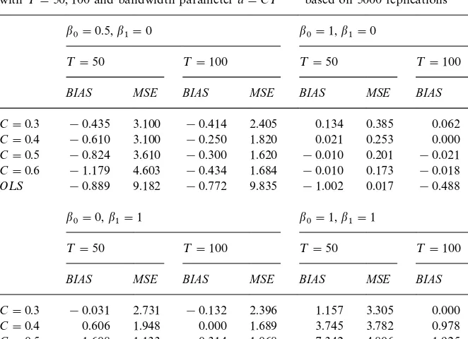
Table 1
Biases and MSEs of nonparametric and OLS estimators of structural break points in model
>
t"qt#(b1qt!b0) 1 (qt*f0)#et,t"1,2,¹
with¹"50, 100 and bandwidth parametera"C¹~1@2based on 5000 replications
b
0"0.5,b1"0 b0"1,b1"0
¹"50 ¹"100 ¹"50 ¹"100
BIAS MSE BIAS MSE BIAS MSE BIAS MSE
C"0.3 !0.435 3.100 !0.414 2.405 0.134 0.385 0.062 0.116
C"0.4 !0.610 3.100 !0.250 1.820 0.021 0.253 0.000 0.036
C"0.5 !0.824 3.610 !0.300 1.620 !0.010 0.201 !0.021 0.018
C"0.6 !1.179 4.603 !0.434 1.684 !0.010 0.173 !0.018 0.013
O¸S !0.889 9.182 !0.772 9.835 !1.002 0.017 !0.488 0.002
b
0"0,b1"1 b0"1,b1"1
¹"50 ¹"100 ¹"50 ¹"100
BIAS MSE BIAS MSE BIAS MSE BIAS MSE
C"0.3 !0.031 2.731 !0.132 2.396 1.157 3.305 0.000 2.470
C"0.4 0.606 1.948 0.000 1.689 3.745 3.782 0.978 2.058
C"0.5 1.608 1.133 0.314 1.068 7.342 4.806 1.925 2.052
C"0.6 2.095 0.600 0.920 0.639 12.880 6.598 3.610 2.465
O¸S 0.837 0.160 0.810 0.074 20.670 7.009 23.83 6.824
Note: All the values in this table must be divided by 100.
LSE converges to 0.25. This appears sensible sincebHincreases asqtincreases to
0.75 and latter decreases. For the other two cases, as the sample size increases, the LSE always performs better as expected, since the MSE of the nonparamet-ric estimator decreases slowly than that of the LSE with the sample size.
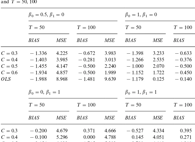
The same Monte Carlo experiment was repeated for model (7), with the same
kernel and bandwidth choicea"C¹~1@2,C"0.3(0.1). The results are provided
in Table 2. Qualitatively, the performance of the estimator is similar to the
situation of"xed regressor, and the same comments given for model (6) apply
here for model (7).
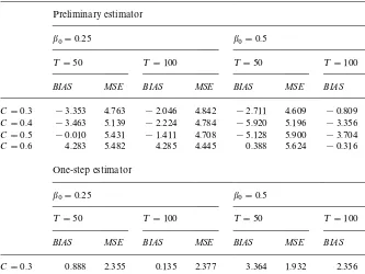
In the second set of Monte Carlo experiments, we have employed the follow-ing autoregressive model with a jump in the mean:
>
t"0.5>t~1#b01(qt*f0)#et, (8)
for two values ofb0, namely 0.25 and 0.50, which correspond to a jump of 0.5
Table 2
Biases and MSEs of nonparametric estimators of structural break points witha"C¹~1@2and OLS estimator based on 5000 replications of the threshold model
>
t"Xt#(b1Xt!b0) 1 (Xt*f0)#et,t"1,2,¹
and¹"50, 100
b
0"0.5,b1"0 b0"1,b1"0
¹"50 ¹"100 ¹"50 ¹"100
BIAS MSE BIAS MSE BIAS MSE BIAS MSE
C"0.3 !1.336 4.225 !0.672 3.983 !1.398 3.233 !0.633 2.825
C"0.4 !1.403 3.985 !0.281 3.013 !1.266 2.535 !0.376 1.434
C"0.5 !1.455 4.147 !0.500 2.240 !1.000 2.070 !0.500 0.679
C"0.6 !1.934 4.857 !0.500 1.989 !1.152 1.722 !0.450 0.434
O¸S !1.988 8.968 !1.481 9.639 !1.179 0.125 !0.140 0.020
b
0"0,b1"1 b0"1,b1"1
¹"50 ¹"100 ¹"50 ¹"100
BIAS MSE BIAS MSE BIAS MSE BIAS MSE
C"0.3 !0.200 4.679 0.371 4.666 !0.527 4.334 0.395 4.087
C"0.4 !0.100 5.296 0.000 4.788 0.145 4.051 0.271 3.075
C"0.5 2.454 6.032 1.715 5.202 2.780 4.418 1.210 2.366
C"0.6 6.980 5.957 4.906 5.728 7.857 5.627 2.614 2.421
O¸S 7.540 1.768 0.475 1.536 19.050 6.364 22.989 6.462
Note: All the values in this table must be divided by 100.
We have employed the kernelsk`(u) and Gaussian for the`regressoratime
and >
t~1 respectively, while the bandwidth choices where a1"C¹~1@2 and
a
2"C¹~1@5withC"0.3 (0.1). The reason to use two di!erent rates of
conver-gence for the bandwidth comes from the well known nonparametric result that the smoother the function, the optimal bandwidth becomes bigger. The results are given in Table 3.
The results are very encouraging, and the estimator, even in this rather complicated model, appears to work very well. Moreover, we clearly observe the gain obtained using the two step algorithm indicated in Section 4. In the
experiment, we have used, as in the initial step, the sample mean of the series>
t,
while in the second step, we employed, as estimators ofk1andk2, the sample
means, using only 0.5¹1@2observations, that is local sample means, to provide
an even more local character to our estimator. Notice that 0.5¹1@2corresponds
roughly to the value¹a
Table 3
Biases and MSEs of nonparametric estimators of structural break points based on 5000 replications of model
>
t"0.5>t~1#b01 (qt*f0)#et, t"1,2,¹
witha
1"C¹~1@2anda2"C¹~1@5,¹"50, 100
Preliminary estimator
b0"0.25 b0"0.5
¹"50 ¹"100 ¹"50 ¹"100
BIAS MSE BIAS MSE BIAS MSE BIAS MSE
C"0.3 !3.353 4.763 !2.046 4.842 !2.711 4.609 !0.809 4.708
C"0.4 !3.463 5.139 !2.224 4.784 !5.920 5.196 !3.356 4.660
C"0.5 !0.010 5.431 !1.411 4.708 !5.128 5.900 !3.704 5.051
C"0.6 4.283 5.482 4.285 4.445 0.388 5.624 !0.316 4.919 One-step estimator
b
0"0.25 b0"0.5
¹"50 ¹"100 ¹"50 ¹"100
BIAS MSE BIAS MSE BIAS MSE BIAS MSE
C"0.3 0.888 2.355 0.135 2.377 3.364 1.932 2.356 1.853
C"0.4 2.194 2.469 0.998 2.340 2.658 1.713 2.052 1.601
C"0.5 5.523 2.897 4.085 2.441 3.164 1.798 1.350 1.636
C"0.6 7.816 3.181 7.016 2.641 4.008 1.917 2.054 1.671 Note: All the values in this table must be divided by 100.
Acknowledgements
Research funded by`DireccioHn General de Ensen8anza Superiora(DGES) of
Spain, reference number: PB95-0292. We are grateful to Inmaculada Fiteni for carrying out the numerical work in Section 5.
Appendix A
Let us introduce some notation. From now on, for any functionq:Rp`1PR,
q
(m)(z)"Rmq(z)/Rzmr and :baq(z) dz":ba[:Rpq(z)<p`jEr1dzj] dzr where z"(z1,
z
2,2,zp`1)@. Also,h"(¹ap`1)1@2,dKj(t),WK 0(f0(j)#tah~1) andf(z) as the pdf of
Z
For the sake of presentation we shall prove"rst Theorem 2, assuming that
j as the solution to
Rg
By Propositions B.4 and B.5 of Appendix B Theorem 5.1 of Robinson (1983),
RY
1j(t),R2j(t),R3j(t) andRY4j(t) are o1(h~2) forj"1,2,N. Thus, (A.1) follows if
h2[r
By Propositions B.1 to B.3, E[h2r
j(t)]"a(0j)k~(1)(0)t2/2#o(t2), while by
Propositions B.4}B.7 and the asymptotic uncorrelation at two di!erent points,
Cov[h2r
to prove the convergence of the"nite dimensional distributions and tightness.
For "xed t1,t2,2,tl3[!M,M]N, by Lemma 7.1. of Robinson (1983), the
asymptotic independence of the kernel regression estimator at two di!erent points and Cra`mer}Wold device,
Next, tightness. By Bickel and Wichura (1971), it su$ces to prove that
∀u
which, by the triangle inequality, will be su$cient if∀j"1,2,N
Pr
G
supwhich holds by Theorem 12.3 of Billingsley (1968), after observing that by
Proposition B.8, lim
and the continuous mapping theorem. But, by Robinson (1983),
6Nj
which converges to zero since sup
jsupfDNj(f)D"O1(a) and Da(1)0 D'Da(2)0 D. Thus,
fK(j)follows similarly. Repeating the same arguments, we have that
Dropping the subscript 1, by standard kernel manipulations and Propositions
and hence, it su$ces to prove that arg max
@t@x1c\(t)"O1(h~1) to conclude.
By Propositions B.1}B.3, and becausea2&h~1by B5,
g6(t)"E(r(t))"(C
(1)(0))"O1(h~1) by standard kernel manipulations. Then
tQ"O
1(h~1), and thustK1"O1(h~1). h
Proof of Corollary 1.(a) Because the additive form of the objective function, that
is +Ml
/1WK l(f)2and we have only changed the kernel function k(u) by kI(u) for
those coordinates responsible of the jump, then by similar arguments to those
employed in Theorem 1, fK
o
The remainder of the proof is identical to that of Theorem 2, and thus is omitted.
(b) The proof is identical to that of Theorem 2(b), and thus is omitted. h
Proof of Corallary 2. By Prakasa Rao's (1981) Theorem 4.5.6.,
x(H!xH"O
1(g~1), where g"(¹ap`2)1@2. Because Rf(xH)/Rx"0,
f(xH)!f(x(H)"O
1(g~2) by de"nition of xH and f()) possesses "nite second
derivatives. Applying the Lemma below, the di!erence of the objective functions
when evaluated at zH(f)"(xH@,f)@ or z(H"(x(H@,f)@ is O
1(h~1). From here, the
Corollary follows proceeding as in the proof of Theorem 2.
corresponds to a maximum where tHis the solution toa0Rg(t)/Rt"0. Then,
tKP$ tHif (A.2) holds. Observe that this agrees with the results of Theorem 2,
where f
By Propositions B.4 and B.5 and a routine extension of Theorem 5.1 of
Robinson (1983), R
j(t)"o1(h~2), j"1,2, 6. Thus, (A.2) follows if
h2r(t)8%!,-:N g(t) on C(!R,R). But, this is the case by similar, if not easier, arguments to those employed in Theorem 2, after observing that by Proposi-tions B.9}B.12.
by Propositions B.4}B.7. Then, we conclude the proof of part (a).
(b) The proof is identical to that of Theorem 2(b), and thus is omitted. h
and thus, withc\(t)"r2(t)#2r(t) (a0#h~1), we have that
K
arg max@t@x1
c((t)!arg max
@t@x1
c\(t)
K
"O 1(h~1).So, it su$ces to prove that arg max
@t@x1c\(t)"O1(h~1) to conclude.
By Propositions B.9}B.12,g6(t)"E(r(t))"d~1C
1t21(t'0)#dC1t21(t)0)
whereC1"a
0k~(1)(0)/2. De"nec6(t)"g6(t)2#2(a0#h~1)g6(t). Then, by
mimick-ing the arguments of the proof of Theorem 1, we obtain thattK"O
1(h~1). h
Proof of Corallary 3. The proof follows by identical arguments of those em-ployed in Theorem 4, after one observes that, by Propositions B.9}B.12,
E (h2r(t))"a0f2(k2)
2f
1(k2)
k~(1)(0)t2#o (1)
whereas, by Propositions B.4}B.7,
Cov(h2r(t1),h2r(t2))"t
1t2m(1)p2e
C
1
f 1(k2)
# 1
f 2(k1)
D
"2t1t2m(1)p2e
C
1 f1(k2)
D
.
h
Appendix B
In the following propositions we assume that, without loss of generality,
t'0, (the caset(0 is similar). Also, we denote byf
0anda0the break point
and its size respectively. De"neg6(z)"f(x)g(z),SB(z,
it)"KB(a~1(z!iu(t)))!
KB(a~1(z!
iu(0))) whereiu(t)"iz0(f0#tah~1) withiz0(f)"(iz01,2,iz0(r~1),
f,
iz0(r`1),2,iz0(p`1))@ and e0 is a p]1 vector of zeroes with a 1 in the
rth position. Propositions B.1}B.8 are proved under the assumptions of
Theorem 2, while Propositions B.9}B.12 under those of Theorem 4. Dropping
the subscriptsi,
Proposition B.1. E[P`(t)]"[g6(1)(z
0)#a0f(1)(x0)]tah~1#O(a2t2h~2).
Proof. According to (1),
E[P`(t)]" 1
ap`1
P
=~=
[g6(z)#a
0f(x)]S`(z,t)dz.
Proposition B.2. E[P~(t)]"!a
By a change of variable and Bochner's (1955) Theorem, the integral is
a0
P
0Proof. The left side of the above equation is
2
Proposition B.5. CovMFB(t1),FB(t2)N"h~4f(x
0)t1t2m(1)#o (t21t22h~4).
Proof. By Lemmas C.6 and C.8 as in Proposition B.4, since f()) is twice
continuously di!erentiable,mB(z)"1 andp2
B(z)"0 in this case. h
Proposition B.6. CovPB(t1),FB(t2)"h~4f(x
0)t1t2mB(z0)m(1)#o(t21t22h~4).
Proof. The left side of the above equation is
2
h4
T
+
i/1
+
j;i
CovMm(Z
i)SB(Zi,t1),SB(Zj,t2)N
#¹
h4CovMm(Zi)SB(Zi,t1),SB(Zi,t2)N.
Then, by Lemmas C.6 and C.8 as in Proposition B.4 or B.5. h
Proposition B.7. For i, j"1, 2, CovMPB(
it1),PY(jt2)N"o(it21jt22h~4),
CovFB(
it1),FY(jt2)"o(it21jt22h~4), CovPB(it1),FY(jt2)"o(it21jt22h~4).
Proof. By Lemmas C.7 and C.9. h
Dropping the superscriptsi,
Proposition B8. lim
T?=h4Var[PB(t1)!PB(t2)])CDt1!t2D2 and
lim
T?=h4Var[FB(t1)!FB(t2)])CDt1!t2D2.
Proof. By Propositions B.4 and B.5. h
For the next four Propositions, let us introduce the following notation. For
i"1, 2, denoteg(z)f
i(x0) asg6i(z).
Proposition B9. E[P`(t)]"!12[g62(z
0)#a0f2(x0)]k~(1)(0)t2h~2#O(a2t2h~2).
Proof. According to (8), by Lemma C.3
E [P`(t)]" 1
ap`1
P
=~=
[g62(z)#a
0f2(x)]S`(z,t) dz,
then apply Lemma C.2 as in Proposition B.1. h
Proposition B.10.
E[P~(t)]"!(a0f2(x0)#f0(x0)g(z0))k~(1)(0)t2
2h2 !
g61(z
0)k~(1)(0)t2
2h2
#O
A
t2a2Proof. Using the same arguments of Proposition B.2, by Lemma C.3, and
recalling thatf
0(x)"f2(x)!f1(x),
E[P~(t)]" 1
ap`1
P
q0`tah~1
q0
(a0f
2(x)#g(z)f0(x))K~
A
z!u(t)
a
B
dz!g61(x0)k~(1)(0)t2
2h2 #O
A
t2a2
h2
B
. hProposition B.11. E[F`(t)]"!f
2(x0)k~(1)(0)t2h~2/2#O (a2t2h~2).
Proof. By Lemma C.3, as in Propositions B.9 and B.10, by continuity off 2())
after observing thatg62(z) isf2(x) anda0"0. h
Proposition B.12. E [F~(t)]"!f
0(x0)k~(1)(0)t2/2h2!f1(x0)k~(1)(0)t2/2h2#
O (a2t2h~2).
Proof. By Lemma C.3, as in Propositions B.9 and B.10, by continuity of both
f
1(x) andf0(x) after replacingg61(z) anda0byf1(x) and 0 respectively there. h
Appendix C
The following lemmas are based on the same assumptions as those of Theorem 2. It is also worthy to mention that the reason in Lemmas C.5, C.7 and C.9 to have, say
it1andjt2, is because in Corollary 3, we evaluate the kernels
K`()) andK~()) at two di!erent points.
Lemma C.1. Letq:Rp`1PRbe a continuous function. Then,
1
ap`1
P
=~=
q(z)SB(z,t) dz"o(1).
Proof. Using a change of variable, the left side of the above equation is equal to
P
= ~=G
q
AA
au#ate0h
B
#z0B
!q(au#z0)H
KB(u) du"o(1),by Bochner's (1955) Theorem. h
Lemma C.2. Letq:Rp`1PRbe twice continuously diwerentiable function.If the kernel functionsKB())are symmetric,then
1
ap`1
P
=~=
q(z)SB(z,t) dz"q (1)(z0)
at
h#O
A
a2t2Proof. By Taylor's expansion ofq(z)
by Lemma C.1 and where the second equality comes because the functionq(1)())
is twice continuously di!erentiable for all coordinates di!erent than therth one,
and the third equality by assumption B5. h
The next lemma will be useful in the case where the time is responsible of the break but it is not a regressor of the model, that is the model considered in Section 4.
Lemma C.3. Letq:Rp`1PRbe twice continuously diwerentiable function.If the kernel functionsKB())are symmetric,then
1
Proof. The left side of the above equation is
Lemma C.4. Let q:Rp`1PR be a twice continuously diwerentiable function.
Proof. Without loss of generality, assume that 0(t
1(t2. After a change of
by MVT and Bochner's (1955) theorem. The lemma follows because m
P
t1@hbecausekB(0)"0. Also by similar, if not easier, arguments
¹
Proof. Without loss of generality, assume that 0(
it1(jt2. After a change of
Lemma C.7. Letq
1())andq2())be as in Lemma C.4. Then, T
+
i/1
+
j;i
Cov [q
1(Zi)SB(Zi,l
1t1),q2(Zj)SY(Zj,l2t2)]"O
A
¹a2(p`1)
h2
B
.Proof. By a routine extension of Lemmas 8.2 and 8.3. of Robinson (1983). h
Lemma C.8. Letq
1())and q2())be as in Lemma C.4. Then,
¹
h4Cov [q1(Zi)SB(Zi,t1),q2(Zi)SB(Zi,t2)]"
1
h4f(x0)q1(z0)q2(z0)t1t2m(1)
#o
A
1h4
B
.Proof. By Lemma C.2, E (q
j(Zi)SB(Zi,tj))"O(ap`2/h), j"1, 2. Then, by
Lemma C.4. h
Lemma C.9. Letq
1())andq2())be as in Lemma C.4. Then,
¹
h4Cov [q1(Zi)SB(Zi,it1),q2(Zi)SY(Zi,jt2)]"o
A
1
h4
B
.Proof. By Lemmas C.2 and C.5. h
References
Andrews, D.W.K., 1993. Testing for structural instability and structural change with unknown change point. Econometrica 61, 821}856.
Andrews, D.W.K., Ploberger, W., 1994. Optimal tests when a nuisance parameter is present only under the alternative. Econometrica 62, 1383}1414.
Antoch, J., Huskova, M., 1997. Estimators of changes. Working paper, Charles University, Praha. Bai, J., 1994. Least squares estimation of a shift in linear processes. Journal of Time Series Analysis
15, 453}472.
Bai, J., 1995. Least absolute deviation estimation of a shift. Econometric Theory 11, 403}436. Bai, J., Perron, P., 1998. Estimating and testing linear models with multiple structural changes.
Econometrica 66, 47}78.
Bickel, P.J., Wichura, M., 1971. Convergence criteria for multiparameter stochastic processes and some applications. Annals of Mathematical Statistics 42, 1656}1670.
Billingsley, P., 1968. Convergence of Probability Measures. Wiley, New York.
Bochner, S., 1955. Harmonic Analysis and the Theory of Probability. University of Chicago Press, Chicago, Illinois.
Brown, R.L., Durbin, J., Evans, J.M., 1975. Techniques for testing the constancy of regression relationships over time. Journal of the Royal Statistical Society Series B37, 149}192. Chan, K.S., 1993. Consistency and limiting distribution of the least squares estimator of a threshold
Chu, J.S., Wu, C.K., 1993. Kernel-type estimators of jump points and values of a regression function. Annals of Statistics 21, 1545}1566.
Delgado, M.A., Hidalgo, J., 1995. Nonparametric inference on structural breaks. Mimeo, Depart-ment of Econometrics, Universidad Carlos III.
Eddy, W.F., 1980. Optimum kernel estimators of the mode. Annals of Statistics 8, 870}882. Eubank, R.L., Speckman, P.L., 1994. Nonparametric estimation of functions with jump
discontinui-ties. Lecture Notes, Vol. 23, Institute of Mathematical Statistics 130}144.
Feder, P.I., 1975. On asymptotic distribution theory in segmented regression problem-identi"ed case. Annals of Statistics 3, 49}83.
Fiteni, I., 1998. Robust estimation of structural break points. Working paper, Universidad Carlos III de Madrid.
Gasser, T., MuKller, H.G., Mammitzsch, V., 1985. Kernels for nonparametric curve estimation. Journal of the Royal Statistical Society Series B47, 238}252.
GyoKr", L., HaKrdle, W., Sarda, P., Vieu, P., 1989. Nonparametric curve estimation from time series. Lecture Notes in Statistics, Vol. 60, Springer, Berlin.
Hansen, B., 1998. Testing for structural change in conditional models. Working paper, University of Winconsin.
Hawkins, D.M., 1977. Testing a sequence of observations for a change in location. Journal of the American Statistical Association 72, 180}186.
Hidalgo, J., 1995. A nonparametric conditional moment test for structural stability. Econometric Theory 11, 671}698.
Hinkley, D., 1969. Inference about the intersection in two phase regression. Biometrika 56, 495}504. Hinkley, D., 1970. Inference about the change point in a sequence of random variables. Biometrika
57, 1}17.
Kim, H.J., Siegmund, D., 1989. The likelihood ratio test for a change point in simple linear regressions. Biometrika 76, 409}423.
MuKller, H.-G., 1992. Change-points in nonparametric regression analysis. Annals of Statistics 20, 737}761.
MuKller, H.-G., Song, K.-S., 1994. Maximin estimation of multidimensional boundaries. Journal of Multivariate Analysis 50, 265}281.
Prakasa Rao, B.L.S., 1981. Nonparametric Functional Estimation. Academic Press, Orlando. Quandt, R.E., 1960. Test of the hypothesis that a linear regression system obeys two separate
regimes. Journal of the American Statistical Association 55, 324}330.
Rice, J., 1984. Boundary modi"cation for kernel regression. Communications in Statistics: Theory and Methods 13, 893}900.
Robinson, P.M., 1983. Nonparametric estimators for time series. Journal of Time Series Analysis 4, 185}207.
Robinson, P.M., 1988. Root-N-consistent semiparametric regression. Econometrica 56, 931}954. Whitt, W., 1970. Weak convergence of probability measures on the function spaceC[0,R). Annals
of Mathematical Statistics 41, 939}944.
Worsley, K.L., 1979. On the likelihood ratio test for a shift in locations of normal populations. Journal of the American Statistical Association 74, 365}367.
Yao, Y.-C., 1987. Approximating the distribution of the maximum likelihood estimate of the change-point in a sequence of independent random variables. Annals of Statistics 3, 1321}1328. Yin, Y.Q., 1988. Detection of the number, locations and magnitudes of jumps. Communications in