Gaussian tests for seasonal unit roots
based on Cauchy estimation and recursive
mean adjustments
Dong Wan Shin
*
, Beong Soo So
Ewha Womans University, Department of Statistics, DeaHyunDong, SeoDaeMoonGu, Seoul, 120-750 South Korea
Received 25 March 1997; received in revised form 13 March 2000; accepted 14 March 2000
Abstract
We propose tests for seasonal unit roots whose limiting null distributions are always standard normal regardless of the period of seasonality and types of mean adjustments. The seasonal models of Dickey, Hasza and Fuller (1984. Journal of American Statistical Association 79, 355}367) (DHF) and Hylleberg, Engle, Granger and Yoo (1990. Journal of Econometrics 44, 215}238) (HEGY) are considered. For estimating parameters related to the seasonal unit roots, regressor signs are used as instrumental variables while recursive sample means are used for adjusting the seasonal means. In addition to normality of the limiting null distributions, in seasonal mean models, the recursive mean adjustment provides the new tests with locally higher powers than those of the existing tests of DHF and HEGY based on the ordinary least-squares estimators. If data have a strong linear time trend, the recursive mean adjustment is a source of both power gains of some tests for local alternatives and power losses of all tests for other alternatives. Limiting normality allow evaluation ofp-values and testing joint signi"cance of subsets of seasonal unit roots. ( 2000 Elsevier Science S.A. All rights reserved.
JEL classixcation: C12; C22
Keywords: Instrumental variable; Normal tests; Sign
*Corresponding author. Fax:#82-2-3277-2614. E-mail address:[email protected] (D.W. Shin).
1. Introduction
Since the pioneering works of Fuller (1976) and Dickey and Fuller (1979), a great deal of attention has been paid to testing for unit roots in economic time series. Economic time series, usually available in monthly or quarterly forms, reveal various kinds of seasonal patterns. As to the issue of random walk versus trend stationarity for yearly or nonseasonal economic time series (Fuller, 1996; Stock, 1994; Hamilton, 1994; and references therein), a major question is whether the main variation of the seasonal time series is a consequence of the nonstationary stochastic seasonality due to the seasonal unit roots or a conse-quence of a deterministic seasonal trend with stationary stochastic seasonality. Dickey et al. (1984) (DHF in the sequel) consider a model that is null
stationary if seasonally di!erenced. Under their model, the time series has all
nonstationary stochastic seasonalities of di!erent frequencies corresponding to
the unit root and all the other seasonal unit roots. Their model considers only seasonal means. Extensions to models containing both seasonal means and a time trend are made by Ahn and Cho (1993) and Cho et al. (1995). Hylleberg et al. (1990) (HEGY in the sequel) and Beaulieu and Miron (1993) point out that seasonal time series can have nonstationary stochastic seasonalities of the
frequencies only corresponding to speci"c seasonal unit roots on the unit circle.
They propose tests which can identify the speci"c frequencies corresponding to
the signi"cant seasonal unit roots. Smith and Taylor (1998a) make extensions
which include seasonal means and seasonal trends. Franses (1994), Ghysels et al. (1996) and Boswijk and Franses (1996) develop tests for seasonal unit roots for
periodic seasonal autoregressive (AR) models in which values of the AR coe$
-cients di!er seasonally.
A special feature of unit root tests for seasonal autoregression is that the limiting null distributions of the unit root tests depend not only on the form of
mean adjustments but also on the period of seasonality. At least"ve di!erent
mean functions may be considered: no mean; a simple mean; seasonal means; a time trend; seasonal means with a time trend. The limiting null distributions of the above-mentioned tests are not normal and are complicated functions of standard Brownian motions. Moreover, the limiting null distributions get more involved because they depend also on the period of seasonality. Hence, in order to have complete test procedures for various mean functions and various periods of seasonality, a large bulk of distributional results and tables of the correspond-ing percentage points are required. Another special feature is that the usual ordinary least squares estimators (OLSEs) adopted by almost all of the above
authors su!er from large downward biases. The biases are, in large part, due to
estimation of the parameters of the mean functions. One serious consequence of the large downward biases of the OLSEs is poor power of unit root tests.
period of seasonality. Both classes of the models of DHF and HEGY are considered. Applications to the periodic models of Franses (1994), Ghysels et al. (1996) and Boswijk and Franses (1996) are obvious. In our new method, the Cauchy estimator developed by So and Shin (1999a) in which the signs of the
regressor variables are used as instrumental variables for estimating the coe$
-cients of seasonal AR models is utilized. The Cauchy estimators allow us to construct asymptotically normal tests for seasonal unit roots. The means are
adjusted by&recursive detrending'developed by So and Shin (1999b) and Shin and
So (1999) in which observations at any time are adjusted for the mean by using observations up to that time point. The recursive mean adjustment provides us with less-biased AR parameter estimates. By adopting the recursive mean adjust-ment, in addition to the smaller biases, we attain limiting normality of the test statistics. The resulting tests for seasonal mean models are shown to be locally more powerful than the existing tests based on the OLSEs. If the mean function consists of a strong linear time trend, then the recursive mean adjustment provides power gains of some tests for some cases of alternative hypotheses close to the null hypotheses but causes power degradation for the other cases.
Limiting null normality of the proposed tests for any seasonality and for any mean function implies several merits. First, the normal tests can be used for a much
wider class of models than the usual nonnormal tests which require di!erent tables
of percentage points for each model and for each period of seasonality. Second, we
can compute thep-values of the test statistics. Since only percentage points of
speci"c probabilities, say, 1%, 2.5%, 5%, and 10%, are usually available for the
usual OLSE-based tests, thep-values of the OLSE-based tests cannot be easily
computed. Availability of thep-values for our tests is a clear advantage over the
OLSE-based tests because thep-values give us detailed information about the
signi"cances of the unit root hypotheses. Third, tests for joint signi"cance of
a subset of seasonal unit roots are possible using the chi-square distributions. The remainder of this paper is organized as follows. In Section 2, the recursive mean adjustment is introduced. In Section 3, based on Cauchy estimation, tests for seasonal unit roots for the model of DHF are developed. In Section 4, tests for seasonal unit roots for the model of HEGY are developed. In Section 5,
extensions to higher-order AR models are made. In Section 6, "nite sample
properties of the proposed tests are investigated through Monte-Carlo experi-ments. In the appendix, proofs of the theoretical results are provided.
2. Recursive mean adjustments
We present our new mean adjustment scheme through a seasonal unit root AR model
y
u
t"out~d#et, (2.2)
where y
t, t"1,2,n, are observations, kt is a mean function, o is the AR
parameter of interest, and d is a positive integer representing the period of
seasonality. The errorse
t are independent and identically distributed with zero
mean and"nite variancep2. We are interested in testing for the seasonal unit
root hypothesis H
0:o"1. For the mean functionkt, we may consider a simple
mean, seasonal means, a simple mean with a trend, seasonal means with a trend, seasonal means and seasonal trends which are given by
k
it are seasonal indicator variables such that dit"1 if
i,t(mod d); d
it"0 otherwise. Among (2.3)}(2.7), the models with seasonal
means (2.4) and the seasonal means with a trend (2.6) are frequently encountered
in practice. If a time series reveals a cycling pattern without time trend,k
tin (2.4)
would be a plausible choice. If a time series reveals a cycling pattern with a linear
trend, then one might consider (2.6). One can also choose one of (2.3)}(2.7) using
the standard model selection criteria such as AIC and BIC.
The traditional methods of DHF, HEGY, and many others are based on the
mean-adjusted observationsy
t!k8t, where the mean functionk8t is constructed
from the OLSEs of the parameters in kt which uses all the observations
My
1,2,ynN. For example, the mean-adjusted estimator of DHF is
o8"+(y
t!y6)(yt~d!y6)/+(yt~d!y6)2, wherey6"n~1+nt/1yt. However, several
authors such as Tanaka (1984), Shaman and Stine (1988), Cruddas et al. (1989), and So and Shin (1999b) point out that this mean adjustment scheme induces
downward biases for estimates ofo. They report that the OLSE has
nonnegli-gible bias especially when the AR root is close to unity or the number of
nuisance parameters is large. For example, when d"1 and k
t"b0, Shaman
and Stine (1988) show that, forDoD(1,
E(o8!o)"!n~1(1#3o)#o(n~1).
We brie#y discuss how the downward bias a!ects powers of the existing tests
based on the OLSE. When DoD(1, the convergence rate of o8 is Jnand the
n~1-order bias is asymptotically negligible. On the other hand, wheno"1, the
convergence rate ofo8isnand then~1-order bias is nonnegligible. Thus the null
distribution ofn(o8!1) is more strongly a!ected than the alternative
distribu-tion of Jn(o8!o) by then~1-order bias. Suppose that we have an estimator
oHwith smaller null bias than o8. Assume that, due to the smaller bias, the 5th
null percentilegHofn(oH!1) is closer to zero by, say, 4 thang8"!13.7, the 5th
null percentile ofn(o8!1) whenn"100 ando"1. This is the case of recursively
mean-adjusted OLSE. NowgH"!9.7. Assume further that, whenn"100 and
o(1, the distributions of Jn(o8!o) and Jn(oH!o) are N(0, 1!o2) and
N(0, i2(1!o2)), respectively. Usually i'1 because reduced-bias estimation
in#ates variances of estimators. Powers of level 5% testsn(o8!1) andn(oH!1)
ato(1 arep8"P[n(o8!1)(!13.7D o]"U[10(0.863!o)/J1!o2] andpH"
P[n(oH!1)(!9.7D o]"U[10(0.903!o)/iJ1!o2], respectively, where
U is the normal distribution function. Therefore, if 0.863!0.04/
(i!1)(o(1, then pH'p8. If 0.863(o(1,pH'p8 regardless of values of
i'1. Ifiis close to one as is the usual case, thenpH'p8 for a wide range ofo. If,
for example, i"1.1, then the range is 0.463(o(1. This example shows
clearly that we can achieve considerable power improvement of unit root tests against stationary alternatives by reducing biases of estimators. We should,
however, admit that the situation is reversed for explosive alternativeso'1 in
whichn(oH!1) becomes less powerful thann(o8!1) due to the reduced bias.
Cruddas et al. (1989) consider a situation in which several AR(1) processes
have a common AR coe$cient and di!erent means. This model is identical to
model (2.1)}(2.2) with mean function (2.4). They apply the method of restricted
maximum likelihood (REML) estimation and conduct Monte-Carlo
simula-tions showing that the REML estimator of the AR coe$cient is substantially
less-biased than the maximum likelihood estimator.
In our seasonal models, we now have two sources of large bias for the OLSE: the existence of unit roots and the large number of nuisance parameters for the seasonal mean functions. We achieve bias reduction by adjusting the mean
through the recursive adjustment of So and Shin (1999b) in whichk
tis estimated
by the OLSE based on the observations My
k(
i are recursively estimated. The recursively adjusted observationsyt!k(t
will be used in Sections 3}5 for estimating the AR coe$cients. Kianifard and
Swallow (1996) discuss applications of slightly di!erent versions of the recursive
residuals for various linear models.
In (2.3)}(2.7), we described the most widely used mean functions. Extensions
to general mean functions are obvious. For model (2.1)}(2.2), let the mean
function bekt"x@tb wherex
t is a sequence of known deterministick-vectors
and b is a k-vector of unknown parameters. Now, the AR coe$cient o is
estimated by an ordinary least squares (OLS)"tting to the recursively demeaned
model
with a less-biased estimator ofobecause, withk(
t~d"x@t~dbK(t!d), the regressor
t~das in the classical approaches, then the regressor is correlated with
the error terme
t due to the correlation betweenbK(n) andet, implying
nonnegli-gible correlation between (y
t~d!k(t~d) ande(t. This, in turn, induces large biases
in estimates ofo. The biases are more severe for models (2.4), (2.6), and (2.7)
because many extra nuisance parameters are estimated. The biases also become
more severe as o gets close to one because the correlation between bK(n) and
e
3. Model of Dickey}Hasza}Fuller
We"rst consider testing seasonal unit root H
0: o"1 for model (2.1)}(2.2).
Given the recursive estimatek(
t, the parametero is estimated from the
mean-adjusted model
y
t!k(t~d"o(yt~d!k(t~d)#e(t. (3.1)
The seasonal unit rootois estimated by using the sign of (y
t~d!k(t~d) as an
instrumental variable. Now, our estimator ofois
o(
called the Cauchy estimator because Cauchy (1836) "rst introduced such an
estimator in a simple linear regression model. This strategy is reviewed in Kotz
and Johnson (1983) in the context of interpolation. The Cauchy estimatoro(
#is also the weighted least-squares estimator for a conditionally heteroscedastic
model y
t"oyt~d#et, E(etDyt~1, yt~2,2)"0, and E(e2t Dyt~1, yt~2,2)"
pDy
t~dD.
Our test for the seasonal unit root is the pivotal statistic of (o(
#!1) de"ned by
a consistent estimator ofp2. Forp(2, we use the OLS variance estimator. Observe
that, under H
is a martingale because, due to the recursive nature ofk(
t~d, sign(yt~d!k(t~d) is
independent ofe
t and hence E[sign(yt~d!k(t~d)etDyj,j(t]"0. Now, by the
martingale central limit theorem (Brown, 1971; Fuller, 1996, p. 235), we get
asymptotic normality of the statisticq(
#.
Theorem 1. Consider model (2.1)}(2.2).Assume thato"1andk
t"0.Then, for
anydand anyp(y
1,2,yt)-measurable mean adjustmentk(t,we haveq(#NN(0, 1),
where N denotes convergence in distribution and p(y
1,2,yt) is the p-xeld
generated byMy1,2,y
tN.
Note that, in (3.1), in addition to y
t~d, yt is also adjusted by
k(
t~d"x@t~dbK(t!d) instead ofx@tbK(t!d). The main reason for adjusting yt by
k(
structure of (3.4) under o"1. However, since y
t is adjusted by k(t~d, the
remaining partkt!k
t~d is not adjusted. If the mean functionkt contains only
seasonal means, thenkt!k
t~d"0 and our scheme of adjustingyt byk(t~d
cre-ates no problem. If k
t contains a time trend, then kt!kt~d does not vanish,
whose e!ect on power performances of test statistics is investigated in Section
6.4. In order to retain the advantage of the limiting normality of the test
statistics, we adjusty
t byk(t~d.
Theorem 1 states that limiting normality of the pivotal statisticq(
#holds for all
positive integersdand for allo3[!1, 1]. This allows us to construct a simple
level (1!a) con"dence intervalo(
#$za@2se(o(#) foro, wherezais thea-percentile
of the standard normal distribution. The asymptotic con"dence interval has
coverage probability (1!a) for allo. On the other hand, the OLSEo(
0cannot be
directly used to construct an asymptotic con"dence interval of the form
o(
0$za@2se(o(0) because limiting distribution of (o(0!o)/se(o(0) is not normal
wheno"1 although it is normal whenDoD(1. Moreover, if mean is adjusted,
the"nite sample distribution ofJn(o(
0!o) foroclose to one is substantially
skewed. By inverting the"nite sample distributions of the OLSEs numerically,
Andrews (1993) constructs con"dence intervals ofo for d"1. In comparison
with Andrews intervals, our con"dence intervals are much simpler and valid for
any positive integerd.
As for the tests based on the OLSE, our test q(
# also has asymptotically
nonzero power against local alternatives of the formo"1!a/n, a'0. Under
such alternatives, the limiting distribution ofq(
#can easily be shown to be of the
form Z!a;
a where Z is a standard normal random variable and ;a is a
strictly positive random variable. Thus, limiting power of size-atestq(
#is strictly
greater than a because lim
n?=P[q(#)!za]"P[Z!a;a)!za]'
P[Z)!z
a]"a.
The sign(y
t) is also used by Burridge and Guerre (1996) in a di!erent context.
They observe that the number of sign changes of an integrated process is smaller than that of a stationary process. They propose to use the number of sign changes as a nonparametric test for a unit root. On the other hand, our method is based on the
parametric estimation which uses the sign(y
t~1) as an instrumental variable.
4. Model of Hylleberg}Engle}Granger}Yoo
4.1. Models and estimation
We present our method through the quarterly model of HEGY. General
d-period model is analyzed after the quarterly model. Consider a fourth order
AR model
t(B)y
whereBis the back shift operator such thatBy
t"yt~1 andt(B) is a
fourth-order polynomial ofB. Assume, without loss of generality, that the constant is 1.
HEGY observe the identity
t(B)"!n0B(1#B#B2#B3)!n2(!B)(1!B#B2!B3)
!(n1B!n
3)(!B)(1!B2)#(1!B4) (4.2)
wheren0,n1,n2, andn3 are determined fromt(B) by comparing both sides of
the identity (4.2). Expressions forni are given in HEGY.
The parametersni determine cycling patterns of the observations y
t. If all
t reveals a#uctuation oscillating two times per year between a random walk
=
t, say, and its negative mirror image!=t. Ift(B) has only a factor (1#B2),
theny
t reveals a#uctuation oscillating once per year between a random walk
and its negative mirror image. Whent(B) has seasonal unit roots at more than
one frequency, y
t reveals a combined #uctuation pattern corresponding to
di!erent seasonal unit roots. See HEGY for other characteristics ofy
taccording
to the seasonal unit roots.
Using (4.2), we reparametrize (4.1) into
z
In (4.3)}(4.4) and in the sequel, we use separating comma &,' in subscripts
wherever requiring clarity and do not use comma elsewhere. Therefore, for
example, bothy
0tandy0,tare used to denote the same quantity and bothq(i#and
q(
i,# are used to denote the same quantity.
One advantage of (4.3) over (2.1)}(2.2) is that we can identify signi"cant
seasonal frequencies of the observations y
t by checkingni"0. HEGY apply
2,t~1, y3,t~1 are almost orthogonal. However, its limiting null distribution
addition, the estimatorsn(
i0 are highly biased when seasonal means or trends are
adjusted. In order to overcome these di$culties, we apply recursive adjustment and
Cauchy estimation for estimatingni. We"rst extend the de"nition of sign(y
it).
Dexnition 1. Let sign
i(yit)"yit/DyitD,i"0, 2; signi(yit)"yit/(y21t#y23t)1@2,i"1, 3,
where it is understood that 0/0"0.
Note that if we de"ne the sign of a complex numberzby sgn(z)"z/DzD, the
complex number sign
1(y1t)#i sign3(y3t) is the same as sgn(y1t#iy3t). One
reason for using the complex signs, sign
1(y1t) and sign3(y3t), fori"1, 3
corre-sponding to the complex root i instead of the usual sign(y1
t) and sign(y3t) is that
the complex signs enable us to establish joint normality of our tests. Another reason is that the tests based on the complex signs have higher power than the tests based on the usual sign.
A mean-adjusted model is (4.3) withy
itreplaced byy8it, wherey8itis the same as
y
itexcept thaty8it is constructed from (4.4) using the recursively mean-adjusted
observationsy
t!k(t instead ofyt. Note thatzt isyt!yt~d. De"ne
v
it"signi(y8it), t"1,2,n,i"0, 1, 2, 3,
and use them as instrumental variables. Let
X The covariance matrix is estimated by
var((n(
#)"p(2(V@X)~1(V@V) (X@V)~1,
wherep(2is the OLSE ofp2. Signi"cance ofn
i is tested by the pivotal statistics
q(
i#"n(i#/se(n(i#), i"0, 1, 2, 3,
where se(n(
i#)"p(cii, cii is the (i#1,i#1) element of (V@X)~1(V@V)(X@V)~1.
We next discuss extensions to generald. Beaulieu and Miron (1993), Franses
(1992), and Taylor (1998) extend the tests of HEGY to the cases d"12 and
d"6. Several other extensions have appeared in Franses and Hobijn (1997)
and Smith and Taylor (1998b, c). Let d be a positive integer. The extended
y
complex signs in De"nition 1 are extended so that sign
0(y0t)"y0t/Dy0tD;
sign
r(yrt)"yrt/DyrtD if d is even; signi(yi,t)#i signi`r(yi`r,t)"(yi,t#iyi`r,t)/
Dy
i,t#iyi`r,tD, i"1,2,r#. Extensions of the testsq(i# are obvious. The limiting null distributions of the test statistics are given below.
Theorem 2. Consider (4.5). For any d and any p(y the standard bivariate normal distribution.
4.2. Hypothesis testing
For testingn
i"0, we use the normal testq(i#,i"0,2,d!1. For testing the
joint hypothesis (n
i,ni`r)"(0,0) which states signi"cance of the seasonal unit
root of frequency 2ni/d, we may use QK
i#"q(2i,##q(2i`r,#, whose limiting null
distribution iss22by Theorem 2, wheres2k is a chi-square random variable with
kdegrees of freedom. However, as observed by HEGY, if explosive processes are
excluded, the alternative hypothesis is (ni(0,ni`rO0) and therefore is partly
one sided. Hence, we can improve the power of the testQK i# by restrictingni to
ni)0. Then the restricted estimator of ni is n8i#"n(
i# if n(i#)0; n8i#"0 if
n(
i#'0. Also, the restricted version ofQKi#isQI i#"q82i,##q(2i`r,#. The limiting null
distribution ofQIi# is a chi-bar square distribution which is a convex
combina-tion ofs21ands22distributions with weightsw
1"limn?=P(n(i#'0)"2~1and
k/0wks2kdenotes a random variable with distribution
function F(x)"+l
k/0wkP[s2k)x], s20"0, if +lk/0wk"1, wk*0, and l is
a positive integer. Now, the joint hypothesis (n
i,ni`r)"(0, 0) is tested by the
statistic QI
i# whose percentage points are available from (4.6) and is given in
Table 1.
Our approach allows us to construct joint tests for seasonal unit roots of di!erent frequencies. LetIbe a subset ofM0, 1,2,rN. Letn(0)"Mn0N;n(i)"Mni,
ni`rN, i"1,2,r#;n(r)"MnrNifdis even. Suppose we want to test the
Table 1
Percentage points of the chi-bar square distribution 0.5s21#0.5s22 p"0.5P[s21)x]#0.5P[s22)x]
p 0.010 0.025 0.050 0.100 0.500 0.900 0.950 0.975 0.990 x 0.006 0.036 0.014 0.049 0.867 3.808 5.138 6.483 8.273
roots eBiC2n*@dfor alli3I. Now, the joint signi"cance is represented by the null
hypothesis H
0: n(i)"M0N for all i3I. The joint hypothesis H0 can be tested
using the statisticsQK
I#"+i|IQK i# orQII#"+i|IQIi#, whereQI 0#"q820# and, ifdis
even,QI
r,#"q82r,#. The limiting null distributions of the testsQK I#andQI I# follow from Theorem 2 and are given below.
Theorem 3. Consider(4.5). UnderH
0:n(i)"M0N for alli3I,for any dand any
p(y
1,2,yt)-measurable mean adjustmentk(t,
(i) q(
i#NN(0, 1)for alli3Iand the limiting distributions are independent,
(ii) QK I#Ns2
2l andQII#N+lk/0(lk)2~ls2l{`k,
wherelis the number of elements inI.Also,l@"lif(dis even, 0NI,andrNI)or(dis odd, 0NI); l@"l!1if (dis even and only one of0or ris inI)or(dis odd and
03I);l@"l!2if dis even and0,r3I.
A simple example consists of testing the joint hypothesis n0"n
1"n2"
n3"0 for the quarterly model. NowI"M0, 1, 2Nandl"3. Thus, the limiting
null distribution of the statistic QI
I#"q820##q821##q822##q(23# is the chi-bar
square distribution (s21#3s22#3s23#s2
4)/8 by Theorem 3(ii). In general, the
limiting null distributions of the one-sided testsQI I#are chi-bar square
distribu-tions and are more complicated than the limiting null distribudistribu-tions of the
two-sided chi-square tests QKI#. However, the one-sided tests QI I# are more
powerful than the two-sided testsQKI#. Percentage points of the chi-bar square
distributions and thep-values of the test statistics can be easily computed using
the chi-square distributions.
5. Extensions to higher-order autoregressive models
A higher-order extension of the model of DHF is
z
t"(o!1)yt~d#h1zt~1#2#hpzt~p#et, (5.1)
where z
t"yt!yt~d. We assume that the characteristic equation
h(B)"1!h1B!2!h
pBphas all roots outside the unit circle. For
e$cient estimators. Thus, we use the e$cient OLSEhK"(hK
1,2,hKp)@which is the
vector of regression coe$cients of z
t~1,2,zt~p in the regression of zt on
y
t~d!k(t~d,zt~1,2,zt~p, t"p#d#1,2,n. Now, the nonstationary
para-meter (o!1) is estimated by applying Cauchy estimation to the model
z8t"(o!1)(y
t~d!k(t~d)#e(t (5.2)
of the residualsz8
t"zt!hK1zt~1!2!hKpzt~p. Thus the Cauchy estimator is
o(
#"1#+sign(yt~d!k(t~d)z8t/+Dyt~d!k(t~dD. The q-statistic q(# for the unit
root is de"ned similarly as in (3.3).
Model (4.5) of HEGY can also be extended to a higher-order model
z
estimated by applying Cauchy estimation to the residual model
z
The test statistics q(
i#,i"0,2,d!1, (QK i#,QI i#), i"1,2,r#, are computed in
the same manner as in Section 4 usingz8
t"zt!hK1zt~1!2!hKpzt~pinstead
ofz
t.
Since the OLSEhK isJn-consistent by Chan and Wei (1988), the limiting null
distributions of the test statistics are the same as those with knownh.
Theorem 4. Consider (5.1). Assume that all the characteristic roots of h(B) lie outside the unit circle and assume o"1.Then, for any d and any p(y
1,2,yt
)-measurable mean adjustmentk(
t, q(#NN(0,1).
Theorem 5. Consider (5.3). Assume that all the characteristic roots of h(B) lie outside the unit circle. Then, for any d and any p(y
Instead of the two-stage "tting of the residual regression (5.2), one can
construct a one-stage instrumental variable estimator for (5.1) by using sign (y
t~d!k(t~d) as an instrument foryt~d!k(t~d andMzt~j, j"1,2,pNas
instru-ments for themselves. Similarly we can construct another instrumental variable
estimator for (5.3) using Msign
Table 2
Empirical sizes (%) of q(
# for testing H0:o"1 against H1:o(1 in model yt!kt"o(yt~d!
kt~d)#e
t!
d"4 d"12
Adjustment (n) 24 48 120 240 480 48 120 240 480
No adjustment 4.3 4.6 4.8 5.3 4.7 3.3 4.2 4.8 5.0
Simple mean 4.4 4.9 4.6 5.2 4.8 2.8 4.4 4.9 5.0
Seasonal means 2.6 3.8 5.1 5.0 4.7 1.1 3.4 4.2 4.6 Simple mean and trend 3.7 4.4 5.0 5.3 5.2 3.1 4.1 5.1 4.7 Seasonal means and trend 2.4 3.6 4.4 5.2 5.2 1.0 3.4 4.6 4.6
!Nominal level"5%, number of samples"10,000, critical value"!1.645.
6. Monte-Carlo study
6.1. Simple models
We"rst consider the DHF model (2.1)}(2.2) and investigate"nite sample sizes
of the testsq(
#. Observationsyt, t"1,2,nare generated from (2.1)}(2.2) using
k
t"0;o"1;n"24, 48, 120, 240, 480; d"4, 12, whereet are standard
nor-mal errors simulated by RNNOA, a FORTRAN subroutine of IMSL (1989).
The initial valuesy0,y~1,y~2,y~3are all set to zero. In Table 2, the empirical
sizes of the testsq(
# with various mean adjustments are given. Each number in
Table 2 represents percentage of 10,000 independent test statisticsq(
# smaller
than!1.645, the 5th left percentile of the standard normal distribution. For the
quarterly case (d"4), the sizes are all between 4.4% and 5.2% and are close to
the nominal level 5% whennis greater than 120 (30 yr). However, whenn"48
or 24, tests adjusted for seasonal means (2.9) and seasonal means with a trend
(2.11) are somewhat undersized. For the monthly case (d"12), forn*240, sizes
are all between 4.2% and 5.1%. Whenn"48 (4 yr), all the tests are downsized.
Generally, we can say that if we have data for more than 20 yr, we have sizes
between 4% and 5.2% for all of the"ve mean adjustments and ford"4, 12.
We next compare the empirical powers of our tests q(
# with those of the
OLSE-based testsq(
0. We consider two adjustments of seasonal means (2.9) and
seasonal means with a trend (2.11). Datay
tare generated from model (2.1)}(2.2)
withkt"0,o"0.95, 0.9, 0.8, 0.7 andn"48, 120, 240, 480. Number of repli-cations is 10,000. Table 3 presents the percentages of the test statistics smaller than the left 5th percentiles of the null distributions of the corresponding test
statistics. The 5th percentile forq(
#is!1.645 for all cases. The 5th percentiles for
q(
Table 3
Empirical powers (%) of q(
# and q(0 for testing H0:o"1 against H1:o(1 in model y
t!kt"o(yt~d!kt~d)#et!
Seasonal means Seasonal means and trend
q(
120 0.90 19.1 34.0 15.8 18.3 18.1 25.4 15.7 15.8
120 0.80 57.3 68.8 29.7 40.3 52.1 56.8 29.7 35.6
120 0.70 92.1 91.1 51.1 61.6 88.5 82.3 51.3 56.4
240 0.95 18.2 35.0 15.5 24.5 17.6 27.4 15.7 21.6
240 0.90 55.3 71.6 29.7 50.3 50.3 57.8 29.8 47.0
240 0.80 99.6 98.7 74.8 88.8 99.0 95.3 74.1 84.9
240 0.70 100.0 100.0 97.9 98.9 100.0 99.8 97.8 98.1
480 0.95 53.8 73.0 28.8 55.1 47.8 59.2 29.1 51.4
480 0.90 99.2 98.6 72.9 91.9 98.4 95.8 72.9 88.4
480 0.80 100.0 100.0 100.0 100.0 100.0 100.0 100.0 100.0 480 0.70 100.0 100.0 100.0 100.0 100.0 100.0 100.0 100.0
!Nominal level"5%; number of samples"10,000; critical value ofq(
c"!1.645. Critical values ofq(
oforn"(48,120,240,480) are (!4.18,!4.10,!4.06,!4.05) for (d"4,k(t"seasonal means); (!4.39,!4.34,!4.29,!4.27) for (d"4,k(
t" seasonal means and trend); (!6.20,!5.86, !5.83,!5.82) for (d"12,k(
t" seasonal means); (!6.02,!6.01,!5.98,!5.95) for (d"12,k(
t"seasonal means and trend).
seasonal meansk
tin (2.4). For a model with seasonal means and a trend (2.6), we
use the empirical 5th percentiles of 10,000 values ofq(
0simulated witho"1. For
almost all cases considered here, we see that our testsq(
#have higher powers than
q(
0. Better powers ofq(#overq(0are more evident ford"12 than ford"4, which
is a consequence of reduced-bias estimation of o using the recursive mean
adjustments (2.8)}(2.12).
We next consider the quarterly model (4.3) of HEGY. We compare our tests
q(
0#, q(2#, andQI 1#with the corresponding testsq(00,q(20, andQK10of HEGY based
on the OLSE. The statistics (q(
00, q(0#), (q(20, q(2#), and (QI10,QK1#) test for signi"
-cance of n0,n1, and (n1, n3), respectively. Datay
t are generated from model
(4.3) withni"0,$0.02,$0.04,$0.08,$0.12, i"0, 1, 2, 3 andn"120. The
test statistics are adjusted for the seasonal meansktof (2.4). The nominal level is
5%. The 5% critical values ofq(
Table 4
Empirical size (%) and power (%) of the tests for model (4.3) adjusted for means!
n0 n2 n1 n3 q(
00 q(0# q(20 q(2# QK10 QI1#
0 0 0 0 4.3 4.4 4.8 4.4 5.0 4.3
0 0 0 0.02 4.0 4.7 4.6 4.7 7.6 9.8
0 0 0 !0.02 4.6 4.6 4.6 4.6 7.0 9.8
0 0 !0.02 0 4.5 4.6 4.7 4.8 7.2 8.1
0 0 !0.02 0.02 3.9 4.5 4.6 4.5 8.7 12.3
0 0 !0.02 !0.02 4.2 4.7 4.6 5.2 8.3 11.6
0 !0.02 0 0 4.1 4.9 7.1 9.8 5.5 4.7
0 !0.02 0 0.02 4.1 4.5 7.3 10.1 7.0 10.0
0 !0.02 0 !0.02 4.8 4.7 6.3 9.4 6.7 9.7
0 !0.02 !0.02 0 4.5 4.8 7.2 10.1 7.3 8.1
0 !0.02 !0.02 0.02 4.2 4.6 7.1 10.5 8.6 12.6
0 !0.02 !0.02 !0.02 4.2 5.0 6.6 9.7 8.5 12.1
!0.02 0 0 0 6.7 9.3 4.3 4.9 5.2 4.1
!0.02 0 0 0.02 6.1 9.5 4.8 4.8 7.4 10.4
!0.02 0 0 !0.02 7.2 10.3 4.2 4.7 6.6 10.1
!0.02 0 !0.02 0 6.7 10.7 4.8 4.4 7.1 7.9
!0.02 0 !0.02 0.02 6.3 10.2 4.7 4.7 8.6 12.2
!0.02 0 !0.02 !0.02 7.1 10.4 4.5 4.8 8.5 11.7
!0.02 !0.02 0 0 6.6 10.4 7.0 10.6 5.4 4.2
!0.02 !0.02 0 0.02 6.3 10.1 7.2 9.8 7.5 10.3
!0.02 !0.02 0 !0.02 6.5 9.7 6.9 10.3 7.2 10.2
!0.02 !0.02 !0.02 0 6.6 10.2 7.0 10.5 7.3 8.1
!0.02 !0.02 !0.02 0.02 6.0 10.3 6.7 9.7 8.5 12.0 !0.02 !0.02 !0.02 !0.02 6.5 10.1 7.1 10.6 9.4 11.9
0 0 0 0.04 3.8 4.7 4.4 4.4 20.2 26.7
0 0 0 !0.04 4.2 4.3 3.9 4.5 20.5 26.5
0 0 !0.04 0 4.1 4.4 4.2 4.5 9.9 10.8
0 0 !0.04 0.04 4.2 4.8 4.5 4.4 15.6 20.8
0 0 !0.04 !0.04 4.4 4.5 4.4 4.9 15.3 20.1
0 !0.04 0 0 4.1 4.3 11.1 16.8 5.2 4.5
0 !0.04 0 0.04 4.5 4.9 11.1 16.9 21.3 34.2
0 !0.04 0 !0.04 4.2 4.7 9.7 16.3 20.5 32.1
0 !0.04 !0.04 0 4.2 4.6 11.4 17.3 9.7 12.4
0 !0.04 !0.04 0.04 4.4 4.8 12.1 18.1 16.1 25.9 0 !0.04 !0.04 !0.04 4.3 4.6 10.9 17.4 15.1 24.2
!0.04 0 0 0 10.4 16.8 4.7 4.3 5.2 4.5
!0.04 0 0 0.04 8.9 15.9 4.7 4.4 21.0 32.2
!0.04 0 0 !0.04 10.9 15.9 3.9 4.3 22.1 34.6
!0.04 0 !0.04 0 11.0 17.4 4.7 4.7 9.8 12.5
!0.04 0 !0.04 0.04 9.2 16.4 4.8 4.8 15.6 25.2
!0.04 0 !0.04 !0.04 10.4 17.1 4.4 4.3 16.3 26.6
!0.04 !0.04 0 0 10.6 17.1 11.4 17.3 5.5 4.7
Table 4 (continued)
n0 n2 n1 n3 q(
00 q(0# q(20 q(2# QK10 QI1# !0.04 !0.04 !0.04 !0.04 11.4 17.9 10.8 17.3 17.0 27.0
0 0 0 0.08 4.0 4.7 4.3 4.8 68.2 79.9 !0.08 !0.08 !0.08 0.08 26.4 36.9 35.6 39.5 51.5 61.0 !0.08 !0.08 !0.08 !0.08 34.6 39.7 27.9 37.4 51.3 59.8
0 0 0 0.12 4.1 5.0 4.3 4.1 92.5 95.6 !0.12 !0.12 !0.12 0.12 56.7 60.5 74.8 66.6 88.4 87.7 !0.12 !0.12 !0.12 !0.12 73.1 66.1 59.0 60.0 88.3 87.0
from Table 1. The 5% critical values of q(
00,q(20, and QK10 are !2.944,!2.918, 6.603 which are interpolated values from HEGY (1990, Tables 1a and b).
In Table 4, percentages of rejected test statistics out of 10,000 independent
tests of n"120 are reported. Numbers below q(
i# and q(i0 are sizes if they
correspond to n
i"0 and are powers if they correspond to niO0,i"0, 2.
Similarly, numbers below QI1# and QK10 are sizes if they correspond to
n1"n
3"0 and are powers otherwise. Even though, the tests are slightly
undersized, the empirical sizes of all the tests are close to the nominal 5% level
for alln
iconsidered here. WhenDniD)0.08, our testsq(0#, q(2#, andQI1#are more
powerful than the corresponding OLSE-based tests q(
00, q(20, and QK 10. When
DniD"0.12, our tests are not more powerful than the OLSE-based tests.
6.2. Tests based on the OLSE and recursive mean adjustment
Power advantage of the proposed Cauchy tests over the existing OLSE-based tests is mainly due to the recursive mean adjustment. Thus, the recursive mean adjustment would also improve powers of the existing tests. We compare power
performance of the proposed tests (q(
#, q(0#, q(2#, QK 1#), the existing OLSE-based
tests (q(
0,q(00,q(20,QK10), and the tests (q(03, q(003, q(203,QK103) based on the OLSE and the recursive mean adjustment. The tests are all adjusted for seasonal means (2.4). The simulation schemes are similar to those for Tables 3 and 4. The statistics (q(
03, q(003, q(203, QK103) are the same as (q(0,q(00,q(20,QK10) except that the recursively adjusted observations are used instead of the observations adjusted by global seasonal means.
In Table 5, rejection frequencies of the testsq(
03, q(0, q(#for the DHF model (3.1)
are reported. The results are based on 10,000 independent replications. As
a critical value ofq(
03, we use the empirical left 5th percentile from 10,000 values
ofq(
03 simulated undero"1. We see that in terms of power performance,q(03is
best,q(
# is intermediate, andq(0is worst. The Cauchy testq(#gains power thanks
to the recursive mean adjustment but loses power owing to lower e$ciency of
the Cauchy estimator than the OLSE especially foro not close to one. Thus,
power performance ofq(
# is in the middle of those ofq(0 andq(03.
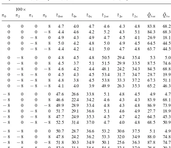
In Table 6, rejection frequencies of the tests for the HEGY model (4.3) are reported. The results are based on 10,000 replications. As critical values of (q(
003,q(203), we use the left 5th empirical percentiles (or right 5th percentile for
QK
103) of 10,000 values of (q(003,q(203) simulated under n0"n1"n2"n3"0. Power performances of the tests are similar to those in Table 5. The tests (q(
003,q(203,QK103) are more powerful than (q(0#,q(2#,QK 1#) which are in turn more
powerful than (q(
00,q(20,QK 10).
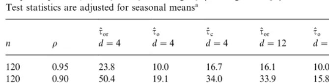
Table 5
Empirical powers (%) ofq(
#andq(0for testing H0:o"1 against H1:o(1 in modelyt"oyt~d#et. Test statistics are adjusted for seasonal means!
q(
03 q(0 q(# q(03 q(0 q(# n o d"4 d"4 d"4 d"12 d"12 d"12
120 0.95 23.8 10.0 16.7 16.1 10.0 9.5
120 0.90 50.4 19.1 34.0 33.9 15.8 18.3
120 0.80 91.8 57.3 68.8 69.0 29.7 40.3
120 0.70 99.8 92.1 91.1 90.7 51.1 61.6
!Nominal level"5%; number of samples"10,000.
recursive mean adjustments would be a good topic for a future research. However, it would require a large number of null distributions and their percentage points for each combination of parameters of seasonal models. On the other hand, our tests based on the Cauchy estimator and the recursive mean adjustment have reasonable power properties and still retain the advantage of standard normal asymptotics for any combination of the parameters of seasonal models.
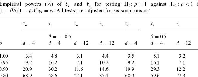
6.3. Higher-order models
We now investigate"nite sample properties of the test statistics for
higher-order models. We"rst consider a model
(1!hB)(1!oBd)y
t"et,
which is equivalent to the DHF model (5.1) with p"1. We compare the test
statistics q(
# and q(0 adjusted for seasonal means. Parameters are set to
d"4, 12;n"120;h"$0.5;o"1, 0.95, 0.9, 0.8, 0.7; and 10,000 replications
are used. The nominal level is set to 5%. The test statisticq(
# is computed from
(5.2) withp"1 by the Cauchy method. The test statisticq(
0 is computed from
OLS-"tting to model (5.1) withp"1. In Table 7, we present rejection
percent-ages of the test statistics. We see that the size of our testq(
#is close to the nominal
level 5% and that ofq(
0is slightly smaller than 5%. The power ofq(#looks greater
than that ofq(
0foro"0.95, 0.9, 0.8. The seemingly higher power ofq(#is partly due to the better performance of the recursive mean adjustment and partly due
to the higher size ofq(
#than that ofq(0. Thus power advantage ofq(#overq(0would
not be as good as in Table 7. Size and power properties of the test statistics for
h"!0.5 are similar to those forh"0.5.
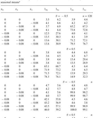
We next consider a higher-order HEGY model of (5.3) with p"1;
n"120, 240; n0,n1, n2"0,!0.08; n3"0;h"$0.5; and 10,000
replica-tions. We compute Cauchy tests (q(
Table 6
Empirical size (%) and power (%) of the tests for model (4.3) adjusted for seasonal means! 100]
n0 n2 n1 n3 q(
003 q(00 q(0# q(203 q(20 q(2# QK103 QK10 QI1#
0 0 0 8 4.7 4.0 4.7 4.6 4.3 4.8 83.8 68.2 79.9
0 0 0 !8 4.4 4.6 4.2 5.2 4.3 5.1 84.3 68.3 79.9
0 0 !8 0 4.9 4.3 4.9 4.7 4.5 4.1 26.9 18.1 23.0
0 0 !8 8 5.0 4.2 4.8 5.0 4.9 4.5 64.5 44.5 56.2
0 0 !8 !8 4.4 4.2 4.1 5.0 4.7 4.8 63.7 44.5 55.7
0 !8 0 0 4.8 4.5 4.8 50.5 29.4 35.4 5.3 5.0 4.7
0 !8 0 8 4.5 3.7 5.1 51.5 29.9 33.5 87.5 74.6 84.3 0 !8 0 !8 4.6 4.2 4.4 48.1 24.2 34.3 84.5 68.8 80.3 0 !8 !8 0 4.5 4.3 4.5 53.4 31.7 34.7 28.7 19.9 25.2 0 !8 !8 8 4.8 3.8 4.5 53.8 33.3 37.2 67.3 51.1 60.0 0 !8 !8 !8 4.1 4.0 3.9 49.9 26.3 35.3 65.2 46.3 57.3 !8 0 0 0 47.6 26.6 33.8 5.1 4.8 4.5 4.9 4.7 4.3 !8 0 0 8 46.6 22.4 34.2 4.6 4.3 4.3 83.9 68.1 79.5 !8 0 0 !8 49.9 28.9 33.4 4.8 4.3 4.8 86.9 73.9 83.7 !8 0 !8 0 51.7 29.1 36.6 5.1 4.6 4.9 27.7 18.9 23.9 !8 0 !8 8 47.7 24.9 35.3 4.5 4.7 4.2 64.5 45.3 56.4 !8 0 !8 !8 52.5 31.4 37.0 4.7 4.0 4.8 68.5 50.9 60.7 !8 !8 0 0 50.7 28.7 36.6 53.2 30.6 37.5 5.1 4.9 4.1 !8 !8 0 8 47.8 24.2 36.2 53.3 32.0 34.9 88.0 74.8 84.5 !8 !8 0 !8 51.8 30.3 34.9 50.1 25.6 36.3 87.8 74.7 84.6 !8 !8 !8 0 52.9 31.1 38.6 54.4 32.4 37.9 28.8 20.3 25.8 !8 !8 !8 8 50.5 26.4 36.9 56.6 35.6 39.5 69.0 51.5 61.0 !8 !8 !8 !8 55.1 34.6 39.7 51.6 27.9 37.4 68.4 51.3 59.8
!Nominal level"5%; number of samples"10,000; period of seasonality"4;n"120.
compute (q(
00, q(20, QK10) from OLS-"tting to model (5.3) withp"1. All tests are
adjusted for seasonal means. In Table 8, we report rejection frequencies of the
test statistics. The nominal level is 5%. Whenn"120, the OLSE-based tests
q(
00 and q(20 are slightly under-sized; the test q(0# is slightly over-sized for
h"!0.5; and the testq(
2# is slightly over-sized forh"0.5. Whenn"240, the
sizes of our tests, as well as the sizes of the OLSE-based tests, get closer to the nominal level within 1% for almost all cases. The seemingly higher powers of Cauchy tests than the OLSE-based tests are due to the two factors of better performance of the recursive mean adjustment and higher sizes of the Cauchy tests.
Table 7
Empirical powers (%) of q(
# and q(0 for testing H0:o"1 against H1:o(1 in model (1!hB)(1!oBd)y
t"et. All tests are adjusted for seasonal means!
q(
0.90 20.9 30.2 11.6 18.6 19.9 29.3 12.2 19.2
0.80 68.9 58.6 27.1 37.1 68.9 59.6 27.3 38.3
0.70 97.1 82.2 56.7 57.1 97.4 82.9 56.8 56.8
!Nominal level"5%; number of samples"10,000;n"120.
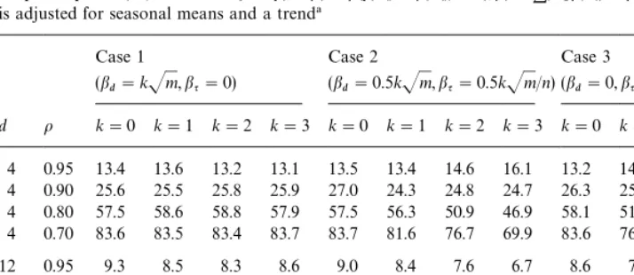
6.4. Power studies for linear trend alternatives
Recall that if the mean function kt contains a time trend component
bqt,bqO0, in the recursive mean adjustment,kt!k
t~d"bqddoes not vanish.
We investigate the e!ect of the unadjusted portion on the power performances
of the proposed tests. We selectkt"+d
i/1bidit#bqt, whereditare the seasonal
dummies. We considerk
n"k]sd(yn)"kJn/d, k"0, 1, 2, 3, where sd(yn)"
Jn/d"Jm is the standard deviation of y
n given by the stochastic trend
y
t"yt~d#et,t"1,2,n,yt"0,t)0. Whenk"3, the deterministic trend is
highly signi"cant compared with the stochastic trend. Noting that
k
n"bd#bqn, we consider three cases: (bd,bq)"(kJm, 0), (0.5kJm,
0.5kJm/n), (0,kJm/n), which are denoted by Case 1, Case 2, and Case 3,
respectively. We letbi"ibd/d,i"1,2,d!1. In Cases 1 and 3, the
determinis-tic mean function consists mainly of seasonal means and of a linear time trend, respectively. In Case 2, the half of the deterministic mean function consists of seasonal means and the remaining half is a linear time trend.
We "rst consider the DHF model y
t!kt"o(yt~d!kt~d)#et in which
e
t are independent standard normal errors; d"4, 12; o"0.95, 0.90, 0.80,
0.70;n"120. In Table 9, the empirical power of the level 5% testq(
#adjusted for
seasonal means and a time trend is presented. Let us "rst investigate the
quarterly case. For Case 1, there is no power loss. For Cases 2 and 3, when
o"0.95, our test q(
# seems to have small power gain as k increases. When
o)0.9, the situation is reversed in that q(
# has substantial power loss as
kincreases especially foro"0.7. Ifk"1, power loss is minor both for Cases
2 and 3, being within 7%. Ifk"2, power loss for Case 2 seems minor but that
Table 8
Empirical size (%) and power (%) of the tests for model (5.3) withp"1. All tests are adjusted for seasonal means!
n0 n2 n1 q(
00 q(0# q(20 q(2# QK10 QI1#
h"!0.5 n"120
0 0 0 3.5 6.2 3.9 4.4 5.0 6.0
0 0 !0.08 4.1 6.6 4.2 4.2 19.3 30.1
0 !0.08 0 3.7 6.9 65.2 67.3 5.5 6.5
0 !0.08 !0.08 4.1 6.4 73.8 72.8 20.0 31.8
!0.08 0 0 12.5 27.6 4.0 4.1 5.4 6.0
!0.08 0 !0.08 13.5 30.3 4.1 3.9 20.1 30.8
!0.08 !0.08 0 13.6 30.1 71.2 72.1 5.7 6.6
!0.08 !0.08 !0.08 13.8 30.9 79.5 76.7 21.2 32.5
h"0.5 n"120
0 0 0 3.8 4.4 4.4 6.8 5.6 6.2
0 0 !0.08 3.6 4.5 4.3 6.7 19.3 29.5
0 !0.08 0 3.9 4.4 13.4 29.4 5.5 5.9
0 !0.08 !0.08 3.8 4.1 13.5 28.9 19.9 30.5
!0.08 0 0 63.1 68.7 4.3 6.4 5.3 6.1
!0.08 0 !0.08 71.9 73.2 3.8 6.5 20.0 31.5
!0.08 !0.08 0 71.5 72.1 13.9 29.3 5.2 6.1
!0.08 !0.08 !0.08 78.3 76.1 14.9 32.3 21.2 32.3
h"!0.5 n"240
0 0 0 4.7 5.6 4.8 4.8 5.3 5.6
0 0 !0.08 4.2 5.7 4.8 4.7 51.3 62.6
0 !0.08 0 4.1 5.6 99.8 98.2 5.4 5.7
0 !0.08 !0.08 4.0 5.7 99.9 98.7 55.2 66.0
!0.08 0 0 42.1 55.8 4.5 4.6 5.1 5.7
!0.08 0 !0.08 43.2 56.9 4.6 3.8 54.9 64.1
!0.08 !0.08 0 43.5 57.1 99.9 98.9 5.3 5.7
!0.08 !0.08 !0.08 46.0 59.2 100.0 99.1 58.3 66.7
h"0.5 n"240
0 0 0 4.1 4.7 4.2 5.6 5.3 5.5
0 0 !0.08 4.4 4.7 4.6 5.6 52.0 62.4
0 !0.08 0 4.4 4.2 43.5 56.3 5.3 5.9
0 !0.08 !0.08 4.3 4.0 45.1 56.7 54.7 64.3
!0.08 0 0 99.9 98.1 4.4 5.6 5.5 5.7
!0.08 0 !0.08 99.9 98.9 4.6 5.7 56.1 66.1
!0.08 !0.08 0 99.9 98.6 46.0 56.9 5.3 5.6
!0.08 !0.08 !0.08 100.0 99.2 47.4 59.2 58.9 67.6 !n3"0; Nominal level"5%; number of samples"10,000; period of seasonality"4.
bigger both for Cases 2 and 3, with o"0.8,0.7. Let us next investigate
Table 9
Empirical power (%) of the testq(
#foryt!kt"o(yt~d!kt~d)#et,kt"+di/1bidit#bqt. The test statistic
is adjusted for seasonal means and a trend!
Case 1 Case 2 Case 3
(bd"kJm,bq"0) (bd"0.5kJm,bq"0.5kJm/n) (bd"0,bq"kJm/n) d o k"0 k"1 k"2 k"3 k"0 k"1 k"2 k"3 k"0 k"1 k"2 k"3
4 0.95 13.4 13.6 13.2 13.1 13.5 13.4 14.6 16.1 13.2 14.7 16.1 17.4 4 0.90 25.6 25.5 25.8 25.9 27.0 24.3 24.8 24.7 26.3 25.4 23.9 22.4 4 0.80 57.5 58.6 58.8 57.9 57.5 56.3 50.9 46.9 58.1 51.5 42.4 33.5 4 0.70 83.6 83.5 83.4 83.7 83.7 81.6 76.7 69.9 83.6 76.6 63.0 49.6 12 0.95 9.3 8.5 8.3 8.6 9.0 8.4 7.6 6.7 8.6 7.1 6.4 6.0 12 0.90 16.7 17.8 17.1 17.1 17.1 15.4 13.2 11.9 17.1 14.2 10.1 8.4 12 0.80 38.3 37.3 39.8 38.5 38.2 34.7 28.4 23.0 38.9 28.8 18.4 12.9 12 0.70 60.9 60.6 59.7 60.4 60.5 54.5 45.2 36.2 60.1 45.3 28.5 19.5
!Nominal level"5%; number of samples"10,000;k"k
n/sd(yn), wheresd(yn)"Jn/d"Jmis the standard deviation ofy
nundero"1 andkt"0;bi"ibd/d,i"1,2,d!1;n"120.
We next consider the HEGY model in whichy
t!ktinstead ofytsatis"es the
quarterly model (4.3) with n1"n
2"n3"n4"n, say, and n"!0.02,
!0.08,!0.16,!0.24; n"120. We consider level 5% tests q(
0#, q(2#, QI1# ad-justed for seasonal means and a time trend. The results are given in Table 10.
For Case 1, all the three tests retain stable powers askincreases. For Case 2,
some tests have power losses in few situations. However, the power losses are
about 10% in worst cases. For Case 3 withk)2, power losses are within about
10% except forq(
0#with (k"2,n"!0.24). For Case 3 withk"3, all the three
tests have some power losses except forq(
0# withn"!0.02,!0.08 for which
substantial power gain is observed.
We can say that the unadjusted linear time trend k
t!kt~d"bqd in the
recursive mean adjustment is a source of both local power gain for the tests
q(
#andq(0#and power deterioration of all the tests against alternative hypotheses
not close to the null hypotheses. If the linear trend is not strong, say, within
$standard deviation of the stochastic trend, then the power loss is not
substan-tial.
Acknowledgements
Table 10
Empirical powers (%) of the tests for model (4.3) with kt"E(yt)"+4i/1bidit#bqt and
n"n
1"n2"n3"n4. The test statistics are adjusted for seasonal means and a trend!
Case 1 Case 2 Case 3
(b4"kJm,bq"0) (b4"0.5kJm,bq"0.5kJm/n) (b4"0,bq"kJm/n)
n k"0 k"1 k"2 k"3 k"0 k"1 k"2 k"3 k"0 k"1 k"2 k"3
q(0#
!0.02 4.7 4.6 4.5 4.5 4.8 7.3 14.8 21.8 5.2 14.6 26.4 32.4 !0.08 14.2 14.3 14.4 14.2 14.6 16.5 21.8 26.2 14.5 21.8 30.2 33.0 !0.16 48.4 49.0 48.5 48.1 48.6 48.6 47.5 46.7 49.1 48.4 46.1 45.0 !0.24 87.4 86.9 86.8 87.6 87.0 85.3 79.8 75.1 87.3 79.8 69.1 63.1
q(
2#
!0.02 10.4 10.6 10.1 10.5 10.2 10.9 9.7 9.1 10.4 9.9 9.0 6.7 !0.08 38.0 37.6 37.7 38.7 38.5 37.3 36.9 34.5 38.2 35.7 31.5 26.5 !0.16 79.7 79.8 79.6 79.0 79.6 78.3 77.3 74.3 79.4 77.0 70.2 62.1 !0.24 95.8 96.0 95.6 96.0 95.7 96.0 94.8 93.7 95.9 95.1 91.5 84.8 QI1#
!0.02 12.1 12.2 12.7 12.6 12.4 13.4 11.1 9.9 12.2 11.3 8.6 6.3 !0.08 61.9 62.2 62.6 62.9 62.7 61.9 59.7 55.9 62.1 59.2 51.6 42.3 !0.16 98.3 98.4 98.3 98.4 98.2 98.2 98.0 97.1 98.4 97.8 95.6 91.6 !0.24 100 100 100 100 100 100 100 100 100 100 100 99.7
!Nominal level"5%; number of samples"10,000;k"k
n/sd(yn), wheresd(yn)"Jn/4"Jmis the standard deviation ofy
nundern"0 andkt"0;bi"ib4/4,i"1,2,4;n"120.
Taylor for their helpful comments. The"rst author is supported by a grant from
Korea Research Foundation (997-001-D00060).
Appendix. Proofs
Proof of Theorem 1. This follows from the martingale central limit theorem
(Brown, 1971). h
Lemma A.1. Let Z
t"(Z1t,2,Zkt)@ be a k-vector AR(1) process dexned by
Z
t"AZt~1#et, where all eigenvalues of A lie inside the unit circle and et is
a sequence of independent identically distributed randomvectors having zero mean. Let X
1t, X2t be sequences of complex-valued random variables and let
=
it"e*hitXit, i"1, 2, where h1, h2 are real numbers in [0, 2p). Assume et is
independent of MX1t,X2
tN, t"1, 2,2. Assume n~1@2=i*nr+N=i(r),
0)r)1,i"1, 2,where=
1(r)and=2(r)are complex-valued Brownian motions
whose real and imaginary parts are Brownian motions dexned on[0, 1].Then
(i) +sgn(X
(ii) ifh1Oh
t is real. Using the fact that, for any positive integerk,
Z
whereDD.DDdenotes matrix norm. Using the fact that sgn(=
)2E[D=
proof remains the same as above except for the fact that, instead of (A.4), we use the following bound
where we have chosenmand N such that n
k!nk~1"m, m N"n,mPR,
Now, we complete the proof by noting that, by (A.4) or (A.5),
)o(Nm)O(n1@2)"o(n~3@2)
and E(D
n))NmO(m1@2)"o(n3@2).
Proof of (iii). This follows from the similar arguments as in the proof of (ii) using
>
t"sgn(=1t=M 2t) instead of>t"sgn(=1t)=M 2t.
Proof of (iv). The proof is similar to that of (i). h
Lemma A.2. Let =
i(r), i"1, 2 be independent standard Brownian motions on
[0, 1].LetA(r)andB(r)bep(=
dent standard normalvariables,whereRe(z)andIm(z)are the real and imaginary parts ofz,respectively.
Proof. By de"nition of the stochastic integral, we haveZ
nNZ, where
are independent N(0,n~1) random variables, the joint moment generating
func-tion of Re(Z
n) and Im(Zn) is
/
n(s1,s2)"E[expMs1Re(Zn)#s2Im(Zn)N]
"exp(!s21/2!s22/2) for all n.
Thus, the result follows. h
Proof of Theorem 2. Let [n@(1)D n@(2)]@be a rearrangement ofnsuch that true value
ofn(1)is zero and no elements ofn(2)are zero. Let [n(@(1)D n(@(2)]@, [X
[V
(1)DV(2)] be corresponding rearranged partitions ofn(c,X, andV, respectively.
For notational convenience, we change the indices in such a way that
M1, 2,2,d
Letkandibe such that they correspond to the paireB*hkof seasonal roots. Let
XH
kt"Xkt#iXit, wherehk"2pk/d, k"0, 1,2,r. By Theorem (2.2) of Chan
and Wei (1988), for somec
k'0,
stationary. Therefore, together with (A.8), Lemma A.1(i) is applicable to give,
n~1V@(1)X
(2)"o1(1), (A.9)
and the upper right blockV@
(1)X(2) ofHn is negligible. Hence
n(
(1)"[V@(1)X(1)]~1[V@(1)e]M1#o1(1)N.
Also, for any k and k@3M0,2,rN, h
k!hk{"2p(k!k@)/dO0, 2p. Hence, by Lemma A.1(ii), the invariance principle, and the continuous mapping theorem,
n~3@2V@(1)X
(1) converges in distribution to a nonsingular distribution whose
o!-diagonals are all zero. Thus,
n(
(1)"[(+DX1tD)~1+sign1(X1t)et,2, (+DXd1tD)~1 +sign
Now, by Lemma A.1(iv),n~1V@
(1)V(2)"o1(1) andn~1V@(1)V(1)"Id1M1#o1(1)N. Hence, together with (A.7) and (A.8),
var((n(
(1))"p(2[V@(1)X(1)]~1[V@(1)V(1)][X@(1)V(1)]~1M1#o1(1)N "np(2diag[(+DX
1tD)~2,2, (+DXd1tD)~2]M1#o1(1)N. (A.11)
From (A.10)}(A.11),
(q(
1,2,q(d1)@"n~1@2p(~1[+sign1(X1t)et,2,+signd(Xd1t)et]M1#o1(1)N.
Choosekfor whichnk"0. We"rst assumehkO0. Letibe a counterpart ofk.
Let XH
kt"Xkt#iXit and =ki"e*hktXHkt. By (A.8) and the weak convergence
result of Kurtz and Protter (1991),
q(
k#iq(i"p(~1n~1@2+sgn(XHkt)et#o1(1) "p(~1n~1@2+sgn(c~1
k =kt)e~*hktet#o1(1) "p(~1[n~1@2+sgn(=
kt)*=M k(t)]#o1(1)N
P
10
sgn(=
k(r)) d=M k(r),
(A.12)
whose real and imaginary parts are independent standard normal random
variables by Lemma A.2. We next consider the case of h
k"0. Then with
Xi
t"=it"0, the arguments leading to (A.12) all hold. Thus, by Lemma A.2,
the distribution (A.12) is again of the form N(0,1)#iN(0,1) and we "nish the
proof, where the two N(0,1) random variables are independent. h
Proof of Theorem 3. By Theorem 2.2 of Chan and Wei (1988), the limiting
distributions (A.12) corresponding to di!erentkare independent and (i) follows.
Result (ii) follow from Theorem 2. h
Proof of Theorem 4. Usingz8t"e
t!Z@t(hK!h), we have
p(q(
#"n~1@2+sign(yt~d!k(t~d)et#Rn,
where R
n"!n~1@2+sign(yt~d!k(t~d)Z@t(hK!h), and Zt"(zt~1,2,zt~p)@.
Now, the result follows from the (hK!h)"O
1(n~1@2) and
n~1+sign(y
t~1!k(t~d)Zt"o1(1),
which is a consequence of Lemma A.1(i). h
Proof of Theorem 5. This follows from Theorem 2 together with the same
References
Ahn, S.K., Cho, S., 1993. Some tests for unit roots in seasonal time series with deterministic trends. Statistics & Probability Letters 16, 85}95.
Andrews, D.W.K., 1993. Exactly median-unbiased estimation of"rst order autoregressive/ unit root models. Econometrica 61, 139}165.
Beaulieu, J.J., Miron, J.A., 1993. Seasonal unit roots in aggregate U.S. data. Journal of Econometrics 55, 305}328.
Boswijk, H.P., Franses, P.H., 1996. Unit roots in periodic autoregressions. Journal of Time Series Analysis 17, 221}245.
Brown, B.M., 1971. Martingale central limit theorems. Annals of Mathematical Statistics 42, 59}66. Burridge, P., Guerre, E., 1996. The limit distribution of level crossings of a random walk and a simple
unit root test. Econometric Theory 12, 705}723.
Cauchy, A., 1836. On a new formula for solving the problem of interpolation in a manner applicable to physical investigations. Philosophical Magazine 8, 459}468.
Chan, N.H., Wei, C.Z., 1988. Limiting distributions of least squares estimates of unstable autoregres-sive processes. Annals of Statistics 16, 367}401.
Cho, S., Park, Y.J., Ahn, S.K., 1995. Unit root tests for seasonal models with deterministic trends. Statistics & Probability Letters 25, 27}35.
Cruddas, A.M., Reid, N., Cox, D.R., 1989. A time series illustration of approximate conditional likelihood. Biometrika 76, 231}237.
Dickey, D.A., Fuller, W.A., 1979. Distribution of the estimators for autoregressive time series with a unit root. Journal of American Statistical Association 74, 427}431.
Dickey, D.A., Hasza, D.P, Fuller, W.A., 1984. Testing for unit roots in seasonal time series with a unit root. Journal of American Statistical Association 79, 355}367.
Franses, P.H., 1992. Modeling seasonality in bimonthly time series. Statistics & Probability Letters 15, 407}415.
Franses, P.H., 1994. A multivariate approach to modeling univariate seasonal time series. Journal of Econometrics 63, 133}151.
Franses, P.H., Hobijn, B., 1997. Critical values for unit root tests in seasonal time series. Journal of Applied Statistics 24, 25}48.
Fuller, W.A., 1976. Introduction to Statistical Time Series. Wiley, New York.
Fuller, W.A., 1996. Introduction to Statistical Time Series, 2nd Edition. Wiley, New York. Ghysels, E.G., Hall, A., Lee, H.S., 1996. On periodic structures and testing for seasonal unit roots.
Journal of American Statistical Association 91, 1551}1559.
Hamilton, J.D., 1994. Time Series Analysis. Princeton University Press, Princeton, NJ.
Hylleberg, S., Engle, R.F., Granger, C.W.J., Yoo, B.S., 1990. Seasonal integration and cointegration. Journal of Econometrics 44, 215}238.
IMSL, 1989. User's Manual. IMSL, Houston, TX.
Kianifard, F., Swallow, W.H., 1996. A review of the development and application of recursive residuals in linear models. Journal of American Statistical Association 91, 391}400.
Kotz, S., Johnson, N.L., 1983. Encyclopedia of Statistical Sciences, Vol. 4. Wiley, New York, pp. 205}207.
Kurtz, T.G., Protter, P., 1991. Weak limit theorems for stochastic integrals and stochastic di!erential equations. Annals of Probability 19, 1035}1070.
Shaman, P., Stine, R.A., 1988. The bias of autoregressive coe$cient estimators. Journal of American Statistical Association 83, 842}848.
Shin, D.W., So, B.S., 1999. Recursive mean adjustment and tests for nonstationarities. Unpublished manuscript, Department of Statistics, Ewha University.
Smith, R.J., Taylor, A.M.R., 1998b. Seasonal unit root tests. Unpublished manuscript, York University, York, UK.
Smith, R.J., Taylor, A.M.R., 1998c. Likelihood ratio tests for seasonal unit roots. Journal of Time Series Analysis 20, 453}476.
So, B.S., Shin, D.W., 1999a. Cauchy estimation for autoregressive process with applications to unit root tests and con"dence interval. Econometric Theory 15, 165}176.
So, B.S., Shin, D.W., 1999b. Recursive mean adjustment for time series inferences. Statistics & Probability Letters 43, 65}73.
Stock, J.H., 1994. Unit roots, structural breaks and trend. In: Engle, R.F., McFadden, D.L. (Eds.), Handbook of Econometrics, Vol. IV. Elsevier, Amsterdam.
Tanaka, K., 1984. An asymptotic expansion associated with the maximum likelihood estimators in ARMA models. Journal of Royal Statistical Society, Series B 46, 58}67.