isprsarchives XL 5 W4 315 2015

(1)

ADVANCES IN IMAGE PRE-PROCESSING

TO IMPROVE AUTOMATED 3D RECONSTRUCTION

A. Ballabeni 1, F. I. Apollonio 1, M. Gaiani 1, F. Remondino 2

1

Dept. of Architecture – University of Bologna, Italy - (andrea.ballabeni, fabrizio.apollonio, marco.gaiani)@unibo.it 2_{3D Optical Metrology (3DOM) unit, Bruno Kessler Foundation (FBK), Trento, Italy}

remondino@fbk.eu, http://3dom.fbk.eu

Commission V, WG 4

KEY WORDS: Pre-processing, Filtering, Matching, Automation, Denoising, RGB to Gray, Color, 3D reconstruction

ABSTRACT

Tools and algorithms for automated image processing and 3D reconstruction purposes have become more and more available, giving the possibility to process any dataset of unoriented and markerless images. Typically, dense 3D point clouds (or texture 3D polygonal models) are produced at reasonable processing time. In this paper, we evaluate how the radiometric pre-processing of image datasets (particularly in RAW format) can help in improving the performances of state-of-the-art automated image processing tools. Beside a review of common pre-processing methods, an efficient pipeline based on color enhancement, image denoising, RGB to Gray conversion and image content enrichment is presented. The performed tests, partly reported for sake of space, demonstrate how an effective image pre-processing, which considers the entire dataset in analysis, can improve the automated orientation procedure and dense 3D point cloud reconstruction, even in case of poor texture scenarios.

1. INTRODUCTION

It is undoubted that image-based 3D reconstruction methods are definitely back and out of the laser scanning shadow. Indeed the integration of automated computer vision algorithms with reliable and precise photogrammetric methods is nowadays producing successful solutions for automated, detailed and accurate 3D reconstruction from image datasets (Snavely et al., 2008; Barazzetti et al., 2010; Pierrot-Deseilligny et al., 2011). This is particularly true for terrestrial applications where we are witnessing the fact that:

• there is a large variety of optical sensors to acquire images with very different performances and thus quality of the delivered imagery;

• it’s constantly growing the impression that few randomly acquired images (or even grab from the Internet) and a black-box software (or mobile app) are enough to produce a decent 3D geometric model;

• automation in image processing is more and more increasing;

• a one-button solution is what non-experts are often seeking to derive 3D models out of inexpensive images.

Due to these reasons, the quality of the acquired and used images is becoming fundamental to allow automated methods of doing their tasks correctly. Motion blur, sensor noise, jpeg artifacts, wrong depth of field are just some of the possible problems that are negatively affecting automated 3D reconstruction methods.

The aim of the present work is to develop an efficient image pre-processing methodology to increase the quality of the results in two central steps of the photogrammetric pipeline:

• the automated alignment of image datasets by:

(i) increasing the number of correct correspondences, particularly in textureless areas;

(ii) tracking features along the largest number of possible images to increase the reliability of the extracted correspondences;

(iii) correctly orienting the largest number of images within a certain dataset;

(iv) delivering sub-pixel accuracy bundle adjustment results.

• the generation of denser and less noisier 3D point clouds.

In this paper the proposed pre-processing pipeline will be evaluated on the image orientation and dense matching issues. The main idea is (i) to minimize typical failure causes by SIFT-like algorithms (Apollonio et al., 2014) due to changes in the illumination conditions or low contrast blobs areas and (ii) to improve the performances of dense 3D reconstruction methods. The pipeline is grounded on the evaluation of many different state-of-the-art algorithms aiming to give solutions at specific problems and adapt the most promising algorithm (from a theoretical viewpoint), thus creating an ad-hoc methodology and an overall solution to radiometrically improve the image quality.

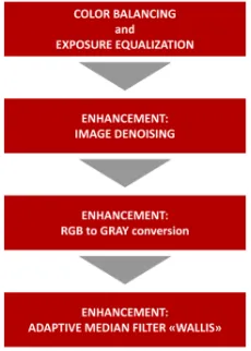
The developed methodology for image pre-processing consists of color balancing (Section 2), image denoising (Section 3), RGB to grey conversion (Section 4) and image content enhancement (Section 5). All the algorithms are tested and applied to raw images, i.e. images as close as possible to the direct camera output.

Figure 1: The proposed image pre-processing pipeline.

2. COLOR BALANCE AND EXPOSURE EQUALIZATION

The aim is essentially to have radiometrically-calibrated images ensuring the consistency of surface colors along all the images (i.e. as much similar as possible RGB values for homologous pixels). Starting from captured RAW images our workflow includes: exposure compensation, optical correction, sharpen and color balance.

(2)

With respect of color characterization, the color targets based technique (Hong et al., 2001) is adopted, using a set of differently colored samples measured with a spectrophotometer. The target GretagMacbeth ColorChecker (McCamy et al. 1976) is employed during the image acquisitions, considering the measurements of each patch as reported in Pascale (2006). The most precise calibration for any given camera requires recording its output for all possible stimuli and comparing it with separately measured values for the same stimuli (Wandell & Farrell, 1993). However, storage of such a quantity of data is impractical, and, therefore, the response of the device is captured for only a limited set of stimuli - normally for the acquisition condition. The responses to these representative stimuli can then be used to calibrate the device for input stimuli that were not measured, finding the transformation between measured CIExyz values and captured RGB values. To find this transformation, several techniques have been developed, including look-up tables (Reinhard et al., 2008).

Summarizing the method for evaluating and expressing color accuracy from this processing includes: a) a physical reference chart acquired under standard conditions; b) a reference chart color space with ideal data values for the chart; c) a means of relating or converting the device color space to the reference chart color space; d) a means of measuring and displaying errors in the device’s rendition of the reference chart. The color

This formula is a new version of the original one (1976) and is more suitable for our uses. It takes into consideration the problem of non-perceptual uniformity of the colors for which ΔE*00 varies the weight of L* depending on where the brightness range falls. Song & Luo (2000) showed that the perceptible and acceptable color differences in complex images presented on a CRT monitor are approximately 2.2 and 4.5, respectively. In our case, the latter value was used as a strict reference for accuracy, defined from perception tests on the results obtained using this value.

Exposure error in f-stops was also evaluated. The ΔE*00 and the exposure error calculations was made using Imatest Studio software version 3.9.

A captured color image containing the GretagMacbeth ColorChecker is neutralized, balanced and properly exposed for the gamma of the reference data set. Using X-Rite ColorChecker Passport Camera Calibration software is generated an ICC profile that was assigned together with the sRGB color space of the RAW image. Before creating ICC profiles, a standard gamma correction (γ = 2.2) is applied, converting all images to the camera’s native linear color space, thus improving the quality of the profiles. A protocol is developed to use the same calibration for groups of images with the same features (i.e., orientation, exposure and framed surfaces) thus to maintain consistency in the process and results. From an operational point of view, the preservation of color fidelity throughout the image processing is ensured by:

- taking pictures in the most possible homogeneous operative conditions (aperture/exposure direction and intensity of light);

- including ColorChecker target inside the photographed scenes in order to correct the image radiometry;

- storing photos in RAW format;

- using an appropriate color space from the beginning of the image processing.

An important and critical issue is the acquisition of the color target. In order to maintain uniform lighting in an external environment, for each image, we need to consider: (i) surfaces illuminated and oriented as the ColorChecker and that presents an angle of incidence with sunlight of approximately 20-45 degrees or (ii) image acquisitions performed with overcast sky. To minimize the light glare, that would give unexpected results in the calibration process, the ColorChecker is normally placed on a tripod with a dark background and orthogonal to the camera optical axis. Finally we verified that a ColorChecker image width of 500 to 1500 pixels is sufficient for ΔE*00 analysis, as suggested also in Imatest user guide.

3. IMAGE DENOISING

Image noise is defined in the ISO 15739 standard as “unwanted variations in the response of an imaging system” (ISO 15739, 2003). It is formed when incoming light is converted from photons to an electrical signal and originates from the camera sensor, its sensitivity and the exposure time as well as by digital processing (or all these factors together). Noise type includes:

• Fixed pattern noise (‘hot’ and ‘cold’ pixels): it is due to always random at any exposure and more influenced by ISO speed.

• Banding noise: it is caused by unstable voltage power and is characterized by the straight band in frequency on the image. It is highly camera-dependent and more visible at high ISO speed and in dark image. Brightening the image or white balancing can increase the problem.

In real-world photographs, the highest spatial-frequency detail consists mostly of variations in brightness (‘luminance detail’) rather than variations in hue (‘chroma detail’):

• Luminance noise is composed of noisy bright pixels that give the image a grainy appearance. High-frequency noise is prevalent in the luminance channel, which can range from fine grain to more distinct speckle noise. This type of noise does not significantly affect the image quality and can be left untreated or only minimally treated if needed.

• Chrominance noise appears as clusters of colored pixels, usually green and magenta. It occurs when the luminance is low due to the inability of the sensor to differentiate color in low light levels. As a result, errors in the way color is recorded are visible and hence the appearance of color artifacts in the demosaicked image.

Under all these considerations, the noise model can be approximated with two components:

a) A signal-independent Gaussian noise modeling the fixed pattern noise (FPN);

b) A signal-dependent Poisson noise modeling the temporal (random) noise, called Shot Noise.

Several denoising methods deal directly with the Poisson noise. Wavelet-based denoising methods (Nowak & Baraniuk, 1997; Kolaczyk, 1999) propose adaptation of the transform threshold to the local noise level of the Poisson process. Recent papers on the Anscombe transform by Makitalo & Foi (2011) and Foi (2011), argue that, when combined with suitable forward and inverse variance-stabilizing transformations (VST), algorithms designed for homoscedastic Gaussian noise work just as well as ad-hoc algorithms based on signal-dependent noise models.

(3)

This explains why the noise is assumed to be uniform, white and Gaussian, having previously applied a VST to the noisy image to take into account the Poisson component.

An effective restoration of image signals will require methods that either model the signal a-priori (i.e. Bayesian) or learn the underlying characteristics of the signal from the given data (i.e. learning, nonparametric, or empirical Bayes’ methods). Most recently, the latter approach has become very popular, mainly using patch-based methods that exploit both local and nonlocal redundancies or ‘self- similarities’ in the images (Lebrun et al., 2012). A patch-based algorithm denoises each pixel by using knowledge of (a) the patch surrounding it and (b) the probability density of all existing patches.

Typical noise reduction software reduces the visibility of noise by smoothing the image, while preserving its details. The classic methods estimate white homoscedastic noise only, but they can be adapted easily to estimate signal- and scale-dependent noise.

The main goals of image denoising algorithms are:

• Perceptually flat regions should be as smooth as possible and noise should be completely removed from these regions;

• Image boundaries should be well preserved and not blurred;

• Texture detail should not be lost;

• The global contrast should be preserved (i.e. the low-frequencies of denoised and input images should be equal);

• No artifacts should appear in the denoised image.

Numerous methods have been developed to meet these goals, but they all rely on the same basic method to eliminate noise: averaging. The concept of averaging is simple, but determining which pixels to average is not. To meet this challenge, four denoising principles are normally considered:

- transform thresholding (sparsity of patches in a fixed basis), - sparse coding (sparsity on a learned dictionary),

- pixel averaging and block averaging (image self-similarity) - Bayesian patch-based methods (Gaussian patch model). Each principle implies a model for the ideal noiseless image. The current state-of-the-art denoising recipes are in fact a smart combination of all these ingredients.

3.1 Evaluated methods and proposed approach

We investigated different denoise algorithms, mostly commercial, namely:

• Imagenomic Noiseware (Imagenomic LLC, 2012;

Petrosyan, & Ghazaryan, 2006);

• Adobe Camera RAW denoise (Schewe & Fraser, 2010);

• Non-Local Bayesian filter (Buades et al. 2005; Kervrann & Boulanger, 2006; Awate & Whitaker, 2006);

• Noise Clinic (Lebrun et al. 2014; Colom et al. 2014;

• Color Block Matching 3D (CBM3D) filter (Dabov et al., 2007b) a color variant of Block Matching 3D (BM3D) filter (Dabov et al., 2007a).

Following results of these experiments, an in-house solution was developed starting from the CBM3D method. CBM3D extends the multi-stage approach of BM3D via the YoUoVo color system. CBM3D produces a basic estimate of the image, using the luminance data and deliver the denoised image performing a second stage on each of the three color channels separately. BM3D is a sliding-window denoising method extending the DCT (Yaroslavsky, 1996) and NL-means algorithms. Instead of adapting locally a basis or choosing from a large dictionary, it uses a fixed basis. The main difference from DCT denoising is that a set of similar patches is used to form a three-dimensional block, which is filtered by using a three-dimensional transform, hence the name collaborative filtering. The algorithm works in two stages: ‘basic estimate’ of

the image and the creation of the final image. A variant of CBM3D from the original Matlab code was implemented, with some customizations. Among these, the most significant is the automatic selection of the parameters based on the ISO sensitivity, the type of camera and stored profiles. Stored profiles (camera, ISO) enable presets for each one of those (can be interpolated, potentially), reading initialization data from the EXIF.

4. RGB TO GRAY

Most image-based 3D reconstruction algorithms are conceptually designed to work on grayscale images instead of the RGB triple. Color to grayscale conversion can be seen as a dimensionality reduction problem. This operation should not be underestimated, since there are many different properties that need to be preserved. In most of the cases isoluminant color changes are usually not preserved during the RGB to Gray conversion. Many conversion methods have been proposed in recent years. They mainly focus on the reproduction of color images with grayscale mediums, with the goal of a perceptual accuracy in terms of the fidelity of the converted image. These kinds of approaches are not designed to fulfill the needs of image matching algorithms where local contrast preservation is crucial during the matching process. This was observed also in Lowe (2004) where the candidate keypoints with low contrast are rejected in order to decrease the ambiguity of the matching process.

RGB to Gray conversion can be done in:

• Color Space (linear or non-linear): the CIE Y method is a widely used conversion, based on the CIE 1931 XYZ color space. It takes the XYZ representation of the image and uses Y as the grayscale value.

• Image Space (called functional): following Benedetti et al. (2012), they can be divided in three groups:

(a) trivial methods: they are the most basic and simple ones, as they do not take into account the power distribution of the color channels. They lose a lot of image information as for every pixel they discard two of the three color values, or discard one value averaging the remaining ones, not taking into account any color properties. Despite this loss, they are commonly used for their simplicity. A typical trivial method is the RGB Channel Filter thatselects a channel between R, G or B and uses this channel as the grayscale value (afterwards called GREEN2GRAY).

(b) direct methods: the conversion is a linear function of the pixel’s color values. Typically, this class of functions takes into account the spectrum of different colors. The Naive Meandirect method takes the mean of the color channels. The advantage, compared to the other trivial ones, is that it takes information from every channel, though it does not consider the relative spectral power distribution of the RGB channels. The most popular of these methods is RGBtoGRAY that uses the NTSC CCIR 601 luma weights, with the formula

Y′= 0.2989R+0.5870G+0.1140B.

Another solution embedded inside Adobe Photoshop uses these specific weights for the channels R, G, and B: 0.4, 0.4, 0.2.

(c) chrominance direct methods: they are based on more advanced color spaces, trying to mitigate the problem related to isoluminant colors. Albeit they are local functions of the image pixels, they assign different grayscale values to isoluminant colors, altering the luminance information using the chrominance information. Chrominance direct methods can be performed either locally (Smith et al., 2008; Kim et

(4)

al., 2009) or globally (Grundland & Dodgson, 2007). Local methods make pixels in the color image not processed in the same way and usually rely on the local chrominance edges for enhancement. Global methods strive to produce one mapping function for the whole image thus producing same luminance for the same RGB triplets and high-speed conversion.

4.1 Evaluated methods and proposed approach We investigated different RGB to Gray methods, namely:

• GREEN2GRAY;

• Matlab RGB2GRAY;

• GRUNDLAND-DODGSON (Grundland & Dodgson, 2007);

• REALTIME (Lu et al. 2012a,b);

• Adobe Photoshop.

Following the tests with the aforementioned methods, a new RGB to Gray conversion technique, named Bruteforce Isoluminants Decrease (BID), was developed. The aim was to preserve the consistency between the images considering the following matching requirements:

‐ Feature discriminability: the method should preserve the image features discriminability to be matched as much as possible;

‐ Chrominance awareness: the method should distinguish between isoluminant colors;

‐ Global mapping: while the algorithm can use spatial information to determine the mapping, the same color should be mapped to the same grayscale value for every pixel in the image;

‐ Color consistency: the same color should be mapped to the same grayscale value in every image of the dataset;

‐ Grayscale preservation: if a pixel in the color image is already achromatic it should maintain the same gray level in the grayscale image;

‐ Unsupervised algorithm: it should not need user tuning to work properly.

BID computes the statistical properties of the input dataset with the help of a representative collection of image patches. It takes in input and analyses simultaneously the whole set of images that need to be matched. Differently from other similar solutions as the Multi-Image Decolorize method (Benedetti et al., 2012), BID is a generalization of the Matlab RGB2Gray algorithm. . BID has its foundation in the statistics of extreme-value distributions of the considered images and presents a more flexible strategy, adapting dynamically channel weights depending on specific input images, in order to find the most appropriate weights for a given color image. BID preserves as much as possible the amount of the conveyed information. The algorithm behind BID tries to maximize the number of peaks obtained in the image converted and to distribute as evenly as possible the amount of tones present in the converted image by evaluating the goodness of fit of the distribution with respect to a rectangular distribution. To calculate the best rectangular fitting we assumed a 0 slope regression line. If the general equation of the regression line is:

β=y−mx

β is equivalent to the average of the histogram points. After calculating the average, the minimum error within all the calculated combinations of channel mixings if sought. The error is calculated as least squares error:

S= ( and blue and for each variation calculates the distribution of the resulting grayscale image and assesses the fitting quality with

respect to a rectangular distribution. Finally BID chooses the mixing that maximizes the number of tones obtained in the converted image. Similarly to Song et al. (2013), BID uses a measurement criterion to evaluate the decolorization quality, i.e. the newly defined dominant color hypothesis. Main disadvantage of BID is the high computational pre-processing cost relieved using sampled patches on each image of the dataset.

5. IMAGE CONTENT ENHANCEMENT

Low-texture surface such as plaster causes difficulties for feature detection such as the Difference-of-Gaussian (DoG) function, which extracts features in pixel level and compares them with adjacent ones and in stereo-matching algorithms. The Wallis filter (Wallis, 1976), is a digital image processing function that enhances the contrast levels and flattens the different exposure to achieve similar brightness in the images. The filter is normally applied in order to optimize image datasets for subsequent image-matching procedures (Baltsavias, 1991; Baltsavias et al., 1996; Seiz et al. 2002; Ohdake et al. 2005; Remondino et al., 2008; MacDonald et al. 2014). Wallis uses two parameters to control the enhancement’s amount, the contrast expansion factor A and the brightness forcing factor B. The algorithm is adaptive and adjusts pixel brightness values in local areas only, contrary to a global contrast filter, which applies the same level of contrast throughout an entire image. The resulting image contains greater detail in both low and high-level contrast regions concurrently, ensuring that good local enhancement is achieved throughout the entire image. The Wallis filter requires the user to accurately set a target mean and standard deviation in order to locally adjusts areas and match the user-specified target values. Firstly the filter divides the input image into neighboring square blocks with a user-defined size (‘window size’) in order to calculate local statistics. Then mean (M) and standard deviation (S) of the unfiltered image are calculated for each individual block based on the grey values of the pixels and the resulting value is assigned to the central cell of each block. The mean and standard deviation values of all other cells in the block are calculated from this central cell by bilinear interpolation. In this way, each individual pixel gets its own initial local mean and standard deviation based on surrounding pixel values. The user-defined mean and standard deviation values are then used to adjust the brightness and the contrast of the input cells. The resulting Wallis filtered image is thus a weighted combination of the original and user-defined mean and standard deviation of the image. The implementation of the filter of Wallis, given the aforementioned factor A and B, can be summarized as follows:

- calculate the enhanced output

(x,y) = S*(input(x,y) – m)/(s + A)+ M*B + m*(1-B)

5.1 Selection of Wallis parameters

The main problem when using the Wallis filter is the correct selection of its parameters. In fact, although several authors reported parameters for successful projects, the filter is more an 'ad-hoc' recipe than an easily deployable system in an automatic photogrammetry pipelines. To overcome this problem, a Wallis parameters characterization study was carried out using three

(5)

different datasets able to encompass the majority of possible surveying case studies. The three datasets consist of:

1. a cross vault characterized by smooth bright-colored plaster; 2.a building facade with porticos with smooth plaster in both

the main and front portico;

3.a Venetian floor, with asphalt and porphyry cubes with a background facade overexposed and an octagonal pillar in the foreground coated with smooth plaster.

For every dataset, three images were matched using a calibrated version (Apollonio et al., 2014) of the SIFT operator available in Vedaldi’s implementation (Vedaldi & Fulkerson, 2010).

a)

b)

c)

Figure 2: Results of the Wallis evaluation on the plaster dataset (1).

From the characterization procedure (Fig. 2), it can be summarized that:

1. the number of tie points found is inversely proportional to the value of the parameter A, but the number of correct matches remains basically stable varying A, which can then be set at high values (6-8);

2. varying the user-specified standard deviation, the number of tie points and correct matches increases substantially linearly up to a value of 100 and then remains constant (Fig.2a); 3. sensor resolution and window size are linearly related and the

increasing of the window size beyond the optimal value does not involve any improvement in either the number of positive matches and in the number of extracted tie points (Fig. 2b); 4. the mean presents optimal values between 100 and 150 with a

decay afterwards (Fig. 2c).

Starting from these observations, a new implementation of the filter was realized to automatically select the filter parameters and achieve the highest possible ratio of corrected matches wrt the number of extracted tie points.

6. EXPERIMENTAL SETUP AND EVALUATION RESULTS

For the evaluation of the implemented methods, different image networks were used with different imaging configurations, textureless areas and repeated pattern/features. The datasets tried to verify the efficiency of the implemented pre-processing pipeline and evaluate its performances. Hereafter, for reasons of space, one peculiar dataset is reported (Building with Porticoes, 35 images – Fig. 3), acquired with a Nikon D3100 (sensor size: 23,1 x 15,4 mm), with a 18 mm nominal focal length. The historical building (19 m height x 10 m width) has three floors characterized by arcades with four aches, pillars/columns, cross vault and plastered wall. The camera was moving along the porticoes, with some closer shots of the columns. The dataset represents an urban test framework and summarizes a typical historical urban scenario. It contains, besides convergent images and some orthogonal camera rolls (ideal for self-calibration), a variety of situations typical of failure cases, i.e. 3D scenes (non-coplanar) with homogeneous regions, distinctive edge boundaries (e.g. buildings, windows/doors, cornices, arcades), repeated patterns (recurrent architectural elements), textureless surfaces and illumination changes.

The performances of the pre-processing strategies previously described are reported using the statistical output of the bundle adjustment (reprojection error), the number of points in the dense point cloud and an accuracy evaluation of the dense matching results. This latter is achieved using a Terrestrial Laser Scanning (TLS) survey as reference (Fig. 4a). Three textureless regions (A1, A2, A3) are identified and, in order to have a reference comparable to the dense matching results, the range data are subsampled to a grid of 5x5 mm. The average image GSD in the three regions of interest is ca 2 mm but the dense matching was carried out using the second-level image pyramid, that is, at a quarter of the original image resolution (i.e. dense point clouds with a sampling resolution of twice the original image GSD).

For every pre-processing method, the Portico dataset is relatively oriented (Fig. 4b) with 4 different tools (Visual SFM, Apero MicMac, Eos Photomodeler and Agisoft Photoscan), trying to keep a uniform number of extracted keypoints and tie points. Then, a dense point cloud is extracted with a unique tool (nFrames SURE) by using (fixing) the same camera parameters for all methods.

6.1 Color balance results

The results of the orientation and dense matching steps are reported in Table 1. The color balancing procedure generally helps in increasing the number of oriented images, except in PS where – as also visible in the next results – the dataset is entirely oriented at every run.

6.2 Image denoising results

After the denoising procedure, the Wallis filtering ia applied to the dataset before running the automated orientation and matching procedures. The achieved adjustment results, according to the different denoising methods, show that more images can be oriented (Table 2) and denser point clouds can be retrieved (Table 3).

(6)

Figure 3: The Portico dataset (35 images) used for the evaluation of the developed image pre-processing pipeline.

Not enhanced Enhanced a) b)

VisualSFM (VSFM)

Numb. oriented images 31 33

BA quality (px) 0.476 0.481

Apero MicMac (AP)

BA reprojection error (px) 0.71 0.85

EOS Photomodeler (PM)

BA reprojection error (px) 0.476 0.481 Agisoft Photoscan (PS)

BA reprojection error (px) 0.512 0.543 Dense Matching (SURE)

Numb. 3D points 1.259.795 1.626.267

Table 1: Bundle adjustment (BA) results and dense matching improvement for the enhancement procedure.

Figure 4: The TLS survey with the 3 textureless regions of interest (a) and the camera network of the Portico dataset (b).

NO DENOISE Adobe CBM3D NL-BAYES NOISE CLINIC IMAGENOMIC

Numb. oriented images 32 35 35 35 35 35

BA quality (px) 0.297 0.476 0.485 0.450 0.694 0.371

BA reprojection error (px) 0.96 0.88 0.88 0.97 0.87 0.93

EOS PhotoModeler (PM)

Agisoft Photoscan (PS)

Table 2: Bundle adjustment (BA) results of the denoising methods applied to the enhanced dataset.

NO DENOISE Adobe CBM3D NL-BAYES NOISE CLINIC IMAGENOMIC Numb. 3D points 998.995 1.308.768 1.456.024 1.456.561 1.428.996 1.346.559

A1 (0,8x1,4m) Ref. pt. cloud:

Numb. 3D

points 1.227 27.508 16.257 31.386 23.419 8.194

(7)

36.294 pts Std Dev

(mm) N/A 12,264 13,613 11,734 12,073 17,219

A2 (0,5x1,9m) Numb. ref. pt.

cloud: 33.868

Numb. 3D

points 495 25.327 17.966 29.632 23.541 7.548

Std Dev

(mm) N/A 11,184 11,735 11,897 11,041 19,002

A3 (2,6x1,3m) Numb. ref. pt.

cloud: 120.222

Numb. 3D

points 32.014 176.478 179.553 183.166 184.835 160.120

Std Dev

(mm) N/A 11,760 12,354 11,443 10,028 10,991

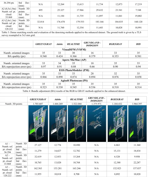
Table 3: Dense matching results and evaluation of the denoising methods applied to the enhanced dataset. The ground truth is given by a TLS survey resampled to 5x5 mm grid.

GREEN2GRAY Adobe REALTIME GRUNDLAND -

DODGSON RGB2GRAY BID

BA quality (px) 0.548 0.424 0.366 0.379 0.353 0.581

EOS PhotoModeler (PM)

Agisoft Photoscan (PS)

Table 4: Bundle adjustment (BA) results of the RGB to GRAY methods applied to the enhanced dataset.

GREEN2GRAY Adobe REALTIME GRUNDLAND -

DODGSON RGB2GRAY BID Numb. 3D points 1.703.607 1.444.269 1.522.044 1.375.971 1.184.432 1.964.397

A1 – Numb. ref.

pt. cloud: 36.294

Numb. 3D

points 27.127 12.776 10.890 N/A 6.863 11.360

Std Dev

(mm) 11,279 14,827 12,782 N/A 15,131 18,834

A2 – Numb. ref.

pt. cloud: 33.868

Numb. 3D

points 32.619 12.853 15.264 N/A 6.520 9.950

Std Dev

(mm) 10,765 13,820 10,768 N/A 12,388 22,287

A3 – Numb. ref.

pt. cloud: 120.222

Numb. 3D

points 162.563 153.281 163.246 N/A 152.923 157.837

Std Dev

(mm) 11,955 10,818 8,708 N/A 8,892 10,820

Table 5: Dense matching results and evaluation of the RGB to GRAY methods applied to the enhanced dataset. The ground truth is given by a TLS survey resampled to 5x5 mm grid.

6.3 RGB to GRAY results

The grayscale conversion (coupled with the Wallis filtering) shows how algorithms are differently affecting the BA procedure (Table 4) as well as the dense matching results (Table 5). It can be generally noticed a larger number of oriented images, better reprojection errors and denser point clouds.

7. CONCLUSIONS

The paper reported some pre-processing methods to improve the results of the automated photogrammetric pipeline. Among the performed tests, a salient example featuring a complex image network and scenario (lack of texture, repetitive pattern, etc.) - and reflecting also the other outcomes achieved in our experiments - was presented. From the results in Section 6 it is

(8)

clear that the pre-processing procedure, with very limited processing time, is generally positively influencing the performances of the orientation and matching tools. The pre-processing is indeed helping in achieving complete orientation results, sometimes better BA reprojection errors (although it is not a real measure of better quality) and, above all, more dense and complete 3D dense point clouds.

According to our tests, the best procedure implies to apply a color enhancement, a denoise procedure based on the BM3D method, the RGB to Gray conversion using the developed BID method and the Wallis filtering. This latter filtering seems to be fundamental also in the orientation procedure and not only at matching level as so far reported in the literature.

The proposed pre-processing pipeline appears particularly suitable and integrable in a fully automated image processing method as:

- the parameters are strictly related to the image metadata (EXIF header) and could be automatically set;

- the pre-processing / filtering considers the entire dataset and it is not image-dependent;

- it is based on criteria related to algorithms employed for automated 3D reconstruction (e.g. keypoint detection) and not on perceptual criteria typically used in image enhancement algorithms;

- it stems from many experiments and merges state-of-the-art methods;

- it gives advantages also for the texture mapping phase. Some final concluding remarks derived by our experiments:

- automated orientation is still an open issue;

- the employed tools for automated image orientation do not provide a unique / standardize type of output;

- there is a lack of repeatability, as already demonstrated in Remondino et al. (2012).

In the near future work we plan to publish all the performed results with more detailed analyses.

REFERENCES

Ancuti, C.O., Ancuti C., Bekaert P., 2010. Decolorizing images for robust matching. ICIP 2010. IEEE International Conference on, Vol Vol. 1, pp. 149-153.

Apollonio, F., Ballabeni, A., Gaiani, M., Remondino, F., 2014. Evaluation of feature-based methods for automated network orientation. ISPRS Archives of the Photogrammetry, Remote Sensing and Spatial Information Sciences, Vol. XL-5, pp. 47-54

Awate, S.P., Whitaker, R.T., 2006. Unsupervised, information-theoretic, adaptive image filtering for image restoration. IEEE Trans. Pattern Anal. Mach. Intell, 28(3), pp. 364-376.

Baltsavias, E. P., 1991. Multiphoto geometrically constrained matching. Ph.D. dissertation No. 9561, Institute of Geodesy and Photogrammetry, ETH Zurich. 221 pp.

Baltsavias, E. P., Li, H., Mason, S., Stefanidis, A., Sinning, M., 1996. Comparison of two digital photogrammetric systems with emphasis on DTM generation: case study glacier measurement. Int. Archives of Photogrammetry, Remote Sensing and Spatial Information Sciences, Vol. XXXI, Part. B4, pp. 104-109.

Barazzetti, L., Scaioni, M., Remondino, F., 2010. Orientation and 3D modeling from markerless terrestrial images: combining accuracy with automation. The Photogrammetric Record, 25(132), pp. 356–381.

Buades, A., Coll, B., Morel, J. M., 2005. A review of image denoising algorithms, with a new one. Multiscale Modeling Simulation (SIAM Interdisciplinary J.), Vol. 4(2), pp. 490-530.

Benedetti, L., Corsini, M., Cignoni, P., Callieri, M., Scopigno, R., 2012. Color to gray conversions in the context of stereo matching algorithms: An analysis and comparison of current methods and an ad-hoc

theoretically-motivated technique for image matching. Machine Vision and Application, Vol. 23(2), pp. 327-348.

Colom, M., Buades, A., Morel, J., 2014. Nonparametric noise estimation method for raw images. J. Opt. Soc. Am. A, Vol. 31, pp. 863-871.

Dabov, K., Foi, A., Katkovnik V., Egiazarian, K., 2007a. Image denoising by sparse 3D transform-domain collaborative Filtering. IEEE Trans. Image Process., Vol. 16(8), pp. 2080-2095.

Dabov, K., Foi, A., Katkovnik, V., Egiazarian, K., 2007b. Color image denoising via sparse 3D collaborative filtering with grouping constraint in luminance-chrominance space. Proceedings of IEEE International Conference on Image Processing (ICIP), Vol.1, pp. I-313 - I-316.

Foi, A., 2011. Noise estimation and removal in MR imaging: The variance-stabilization approach. IEEE International Symposium on BiomedicalImaging: From Nano to Macro, pp. 1809-1814.

Gooch, A.A., Olsen, S.C., Tumblin, J., Gooch, B., 2005. Color2gray: salience-preserving color removal. ACM Trans. Graph., Vol. 24(3), pp. 634-639.

Grundland, M., Dodgson, N.A., 2007. Decolorize: fast, contrast enhancing, color to grayscale conversion. Pattern Recognition, Vol. 40(11), pp. 2891-2896.

Kervrann C., Boulanger J., 2006, Optimal spatial adaptation for patch-based denoising. IEEE Trans. Image Process., Vol. 15(10), pp. 2866-2878.

Kim, Y., Jang, C., Demouth, J., Lee, S., 2009. Robust color-to-gray via nonlinear global mapping, ACM Transactionson Graphics, Vol. 28(5).

Kolaczyk E., 1999. Wavelet shrinkage estimation of certain Poisson intensity signals using corrected thresholds. Statist. Sin., Vol. 9, pp. 119-135.

Imagenomic LLC (2012). Noiseware 5 Plug-In User’s Guide

Lebrun M., Colom M., Morel J.-M., 2014. The Noise Clinic: a blind image denoising algorithm, Ipol Journal, preprint.

Lebrun, M., Colom M., Buades, A., Morel, J.-M., 2012. Secrets of image denoising cuisine, Acta Numerica, Vol. 21, pp. 475-576.

Lowe, D., 2004: Distinctive image features from scale-invariant keypoints. Int. Journal of Computer Vision, Vol. 60(2), pp. 91-110.

Lu C., Xu L., Jia J., 2012. Contrast preserving decolorization. ICCP, 2012 IEEE International Conference on, pp.1-7.

Lu C., Xu L., Jia J., 2014. Contrast preserving decolorization with perception-based quality metrics. International Journal of Computer Vision, Vol. 110(2), pp. 222-239.

MacDonald, L., Hindmarch, J., Robson, S., Terras, M., 2014. Modelling the appearance of heritage metallic surfaces. Int. Archives of Photogrammetry, Remote Sensing and Spatial Information Sciences, Vol. XL(5), pp. 371-377.

McCamy, C.S., Marcus, H., Davidson, J.G., 1976. A color rendition chart. Journal of Applied Photographic Engineering, Vol. 11(3), pp. 95-99.

Makitalo, M., Foi, A., 2011. Optimal inversion of the Anscombe transformation in low-count Poisson image denoising. IEEE Trans. Image Processing,Vol. 20, pp. 99-109.

Nowak, R. Baraniuk, R., 1997. Wavelet-domain ﬁltering for photon imaging systems. IEEE Trans. Image Processing,Vol.8, pp. 666-678.

Ohdake, T., Chikatsu, H., 2005. 3D modeling of high relief sculpture using image based integrated measurement system. Int. Archives of Photogrammetry, Remote Sensing and Spatial Information Sciences, Vol. XXXVI(5-W17), 6 pp.

Pascale, D., 2006. RGB coordinates of the Macbeth ColorChecker. The BabelColor Company, Montreal, Canada.

Petrosyan, A., Ghazaryan, A., 2006. Method and system for digital image enhancement. US Patent Application, Vol. 11(116), pp. 408.

(9)

Pierrot-Deseilligny, M., De Luca, L., Remondino, F., 2011. Automated image-based procedures for accurate artifacts 3D modeling and orthoimage generation. Geoinformatics FCE CTU Journal, Vol. 6, pp. 291-299.

Reinhard, E., Arif Khan, E., Oguz Akyüz A., Johnson G., 2008. Color Imaging Fundamentals and Applications. A. K. Peters: Wellesley.

Remondino, F., El-Hakim, S., Gruen, A., Zhang, L., 2008. Turning images into 3D models - Development and performance analysis of image matching for detailed surface reconstruction of heritage objects. IEEE Signal Processing Magazine, Vol. 25(4), pp. 55-65.

Remondino, F., Del Pizzo, S., Kersten, T., Troisi, S., 2012. Low-cost and open-source solutions for automated image orientation – A critical overview. Proc. EuroMed 2012 Conference, LNCS, Vol. 7616, pp. 40-54

Schewe, J., Fraser, B., 2010. Real World Camera Raw with Adobe Photoshop CS5. Peachpit Press, Berkeley, CA, USA, 480 pp.

Seiz G., Baltsavias E. P., Grün A., 2002. Cloud mapping from ground: use of photogrammetric methods. Photogrammetric Engineering and Remote Sensing, Vol. 68(9), pp. 941-951.

Sharma, G., Wu, W., Dalal, E.N., 2005. The CIEDE2000 Color-difference formula: implementation notes, supplementary test data and mathematical observations. Color Research and Application, Vol. 30(1), pp. 21-30.

Smith, K., Landes, P. E., Thollot, J., Myszkowski, K., 2008. Apparent Greyscale: a simple and fast conversion to perceptually accurate images and video. Computer Graphics Forum, Vol.27(2), pp. 193-200.

Snavely, N., Seitz, S.M., Szeliski, R., 2008. Modeling the world from internet photo collections. Int. Journal of Computer Vision, Vol. 80(2), pp. 189-210.

Song, Y., Bao, L., Xu, X., Yang, Q., 2013. Decolorization: Is rgb2gray() out?, SIGGRAPH Asia 2013 Technical Briefs (SA '13), ACM, New York, 15, 4pp.

Song, T., Luo, M.R., 2000. Testing color-difference formulae on complex images using a CRT monitor. Proceedings of IS&T and SID Eighth Color Imaging Conference, pp. 44-48.

Vedaldi, A., Fulkerson, B., 2010: VLFeat - An open and portable library of computer vision algorithms. Proc.18th _{ACM Intern. Conf. on} Multimedia

Wallis R., 1976, An approach to the space variant restoration and enhancement of images. Proceedings of Symp. Current Mathematical Problems in Image Science, Monterey, Naval Postgraduate School, pp. 329-340.

Wandell, B.A., Farrell J.E., 1993. Water into Wine: converting scanner RGB to tristimulus XYZ. Proceedings of SPIE, Vol. 1909, Bellingham, pp. 92-101

Yaroslavsky, L.P.. 1996, Local adaptive image restoration and enhancement with the use of DFT and DCT in a running window. Proceedings of SPIE, Vol. 2825, Bellingham, pp. 2-13