AN EXPLORATORY SPATIAL ANALYSIS OF SOIL ORGANIC CARBON
DISTRIBUTION IN CANADIAN ECO-REGIONS
S.-Y. Tan a, *, J. Li a
a
Dept. of Geography and Environmental Management, University of Waterloo, 200 University Ave. West, Waterloo, Ontario, Canada N2L 3G1 - [email protected]
KEY WORDS: Climate, Land Cover, Precipitation, Satellite, Soil, Spatial, Temperature, Vegetation
ABSTRACT:
As the largest carbon reservoir in ecosystems, soil accounts for more than twice as much carbon storage as that of vegetation biomass or the atmosphere. This paper examines spatial patterns of soil organic carbon (SOC) in Canadian forest areas at an eco-region scale of analysis. The goal is to explore the relationship of SOC levels with various climatological variables, including temperature and precipitation. The first Canadian forest soil database published in 1997 by the Canada Forest Service was analyzed along with other long-term eco-climatic data (1961 to 1991) including precipitation, air temperature, slope, aspect, elevation, and Normalized Difference Vegetation Index (NDVI) derived from remote sensing imagery. In addition, the existing eco-region framework established by Environment Canada was evaluated for mapping SOC distribution. Exploratory spatial data analysis techniques, including spatial autocorrelation analysis, were employed to examine how forest SOC is spatially distributed in Canada. Correlation analysis and spatial regression modelling were applied to determine the dominant ecological factors influencing SOC patterns at the eco-region level. At the national scale, a spatial error regression model was developed to account for spatial dependency and to estimate SOC patterns based on ecological and ecosystem factors. Based on the significant variables derived from the spatial error model, a predictive SOC map in Canadian forest areas was generated. Although overall SOC distribution is influenced by climatic and topographic variables, distribution patterns are shown to differ significantly between eco-regions. These findings help to validate the eco-region classification framework for SOC zonation mapping in Canada.
* Corresponding author
1. INTRODUCTION
As the largest organic carbon reservoir in ecosystems, soil accounts for more than twice as much carbon storage as vegetation biomass or the atmosphere (Galbraith et al., 2003). Globally, about 30% of soil organic carbon (SOC) is estimated to be preserved in tundra and boreal ecosystems (Lee et al., 2010). In forest ecosystems, the amount of SOC is calculated as the difference between organic carbon inputs and releases. Consequently, due to effective vegetation-soil interactions and decades of accumulation, considerable organic carbon has been stored in forest soils.
The dynamics of such large quantities of organic carbon stored in forest soil not only influence soil fertility and forest productivity, but also partly account for changes in atmospheric carbon concentration (Mishra et al., 2010). Many studies have pointed out that SOC distribution is temperature-sensitive and small fluctuations in SOC could greatly affect atmospheric carbon concentration (Shakiba & Matkan, 2005; Tewksbury & Van Miegroet, 2007). To date, the influence of temperature on SOC distribution remains controversial. In comparison to temperature effects, the impact of precipitation on SOC distribution is usually observed to be dominant and positive. Soils in humid eco-regions usually accumulate more organic carbon (Buringh, 1984), because high levels of soil moisture tend to reduce SOC decomposition rates by slowing and restricting oxygen diffusion processes.
In SOC-landscape modelling, topography is considered to be a dominant influence on pedogenic processes (Tewksbury & Van Miegroet, 2007). Vegetation cover also influences SOC input and distribution through litterfall accumulation. In particular,
SOC distribution is positively related to forest age (Chen et al., 2003), and old-growth forest is more capable of SOC sequestration than young-growth forest (Luyssaert et al., 2008). Moreover, the amount of SOC is influenced by historic land use changes and human disruptions (Galbraith et al., 2003). As a result, policy making and forest resource management necessitates having a solid understanding of SOC distribution and influencing variables.
Recent studies have used geostatistical techniques and spatial regression analysis to incorporate environmental information into SOC mapping, rather than relying on ground soil surveys and in situ measurements (Mishra et al., 2010). These studies are based on two main assumptions. First, specific soil properties (e.g., SOC distribution) vary in space and through time across ecosystems, because different ecological conditions have varying impacts on pedogenic processes (Chen, et al., 2003). Second, ecological factors contribute to SOC-environment relationships unequally and to varying levels in different environments.
In Canada, about 4,690,000 km2
(47% of total area) are covered by intact forest (Lee et al., 2010). This forest-dominant landscape indicates that Canada is one of the vital carbon reservoirs in the world. Consequently, many efforts have been made to estimate Canadian SOC distribution and to model SOC-environment relationships. However, most studies have been conducted at the local scale with limited SOC distribution and SOC-environment modelling conducted at a national or regional scale of analysis. Therefore, the main research goal of this study is to examine spatial patterns of SOC distribution in Canadian forest regions at the eco-region scale and to explore relationships between SOC and various ecological variables.
More specifically, the objectives of this study include:
1. To explore the spatial distribution of SOC levels in Canadian forests in seven eco-regions: the Subarctic, Boreal, Cool Temperate, Subarctic Cordilleran, Cordilleran, Interior Cordilleran, and Pacific Cordilleran, 2. To assess the influence of ecological factors on forest
SOC stock in growing seasons at regional scales of analysis, including elevation, slope, aspect, Normalized Difference Vegetation Index (NDVI), precipitation, and maximum/mean/minimum air temperatures, and
3. To assess how SOC-environment relationships vary geographically with respect to ecological factors.
2. MATERIALS & METHODS
2.1 Study Area
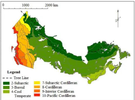
This study focuses on forest covered areas in Canada, excluding tundra areas, grassland, and main water bodies, as shown in Figure 1. Based on ecological responses (e.g., vegetation types, hydrological conditions, and biota) to different climatic regimes, seven eco-climate regions are delineated: Subarctic, Boreal, Cool Temperate, Subarctic Cordilleran, Cordilleran, Interior Cordilleran, and Pacific Cordilleran. The treeline or altitude above which fewer trees grow is located in the Subarctic eco-region, also shown in Figure 1. MacDonald and Gajewski (1992) emphasizes that the tree line is not a specific curve that explicitly separates forested and non-forested areas. Instead, it represents a transitional zone consisting of forest and other northern surface features (e.g., tundra).
Figure 1. Study area of Canadian forest regions
2.2 Data & Data Preprocessing
The Canadian Forest Service (CFS) database consists of field survey data collected before 1991, making it a useful source of historical SOC data. By excluding tundra areas, the remaining 1,317 records in forest regions were used in this study. The SOC stock was measured to a depth of one meter of mineral soil for each soil profile record. A map of the distribution of original SOC sample points is shown in Figure 2.
Long term climate data in growing seasons (April to October) from 1961 to 1991 were collected. Daily 10 km Gridded Climate datasets were provided by the National Land and Water Information Service, Agricultural Canada with the average maximum, mean, and minimum air temperatures (°C) for each
year’s growing seasons calculated. Daily precipitation data (mm) was summed for growing seasons.
Figure 2. The spatial distribution of 1,317 CFS soil samples collected in Canadian forest areas before 1991 by the Canada
Forest Service
In order to obtain complete landmass coverage of seasonal climate data beyond the 60⁰ latitude, data from 34 weather stations across Northern provinces from Environment Canada were collected. Data points were interpolated by Ordinary Kriging and merged by using the ArcGIS Mosaic software tool.
The 16-day NDVI datasets from 1981 to 1991 at 8 km spatial resolution were acquired from the Global Inventory Modeling and Mapping Studies (GIMMS). Other topographic attributes – elevation, slope, and aspect – were derived from a digital elevation model (DEM) provided by CFS. All datasets were re-sampled to 10 km resolution for comparable cell size.
2.3 Spatial Data Analysis
Global and local autocorrelation analyses were applied to test the null hypothesis of spatially independent SOC samples. The global Moran’s I test measures the overall degree of spatial autocorrelation and returns a single value applied to the entire study area to indicate an overall spatial clustered or dispersed pattern (Anselin, 2005). A positive global Moran’s I value suggests the comparability among proximal observations, while a negative value indicates a spatially dispersed pattern. The local spatial autocorrelation analysis highlights four types of local spatial patterns: High (HH), Low-Low (LL), High-Low (HL), and High-Low-High (LF). The HH and LL patterns are known as ‘spatial clusters’ within which the observations have positive Moran’s I values and share similar spatial information. The HL and LH patterns are considered to be ‘spatial outliers’, whose values are significantly different from their neighbours.
In this study, the global and local spatial autocorrelation is measured at both national and eco-region scales. The Subarctic Cordilleran eco-region was excluded, since it contained a small sample of only 14 observations. According to ESRI (2013), the optimal number of samples used to calculate the Moran’s I should not be less than 30.
This study adopted the Incremental Spatial Autocorrelation approach to automatically calculate the global Moran’s I at a series of incremental distances (ESRI, 2013). This entails calculating a Z-score associated with each global Moran’s I value at each distance increment to quantify the strength of The International Archives of the Photogrammetry, Remote Sensing and Spatial Information Sciences, Volume XL-2, 2014
spatial dependency. Significant and positive peak Z-scores signify the spatial scales at which the ecological responses of targeted objects to cluster-patterns are most notable (ESRI, 2013). In particular, the peak Z-scores associated with larger distances indicate general distribution trends (e.g., decreasing SOC stock from coasts to interior continental regions), while the peaks associated with smaller distances could preserve local variations. Thus, the distance where the first peak Z-score occurs was considered to be optimal for the spatial analysis. In this study, the Nearest Neighbour Distance (NND) of each soil sample was calculated. Any sample with a NND three times larger than its standard deviation (SD) was considered as spatial outliers and removed from the dataset (ESRI, 2013).
In order to investigate whether the detected spatial patterns of targeted objects are generated by specific processes, the relationships between SOC and ecological variables at national and eco-region scales were tested based on spatial regression models. The Lagrange Multiplier (LM) test illustrated in Figure 3 was applied to assist with model selection (Anselin, 1988). Given regression equation:
y = α + ρ Wy + β X + ɛ ; ɛ = λ Wɛ + u (1)
where y is the dependent variable, X is a set of independent variables, α is the intercept, β is the parameter, λ is the parameter for an autocorrelated spatial error term, ρ is the parameter for an autocorrelated spatially lagged term, W is the spatial weights, Wy is the spatially lagged component of y, Wɛ is the spatial autocorrelated error terms, and u is the independent and identically distributed (i.i.d.) errors. LM diagnostics are empirical tests with the null hypothesis of λ = 0 or ρ = 0 (Anselin, 1988):
- When the null hypothesis, λ = 0 and ρ = 0, is accepted, a traditional OLS model is the appropriate model specification. - If λ = 0 and ρ ≠ 0 is true, a spatial error model should be
applied.
- If λ≠ 0 and ρ = 0 is true, a spatial lag model should be applied.
Figure 3. (a) Sub-workflow of regression model selection process, and (b) illustration of spatial processes described by
spatial error and lag models (Source: Anselin, 2005)
The spatial lag model is considered to be more appropriate when: (1) the existence of interactions among dependent variable, y , is pronounced, (2) the impacts of nearby dependent variables on yi are greater than those of independent variables,
xi at location i (Anselin, 2005). In contrast, the spatial error
model takes unobservable factors into consideration, suggesting that omitted variables showing certain spatial patterns should account for most of the spatial dependence of estimation errors.
The last part of this study employs a multi-criteria analysis to produce a predictive map of SOC in Canadian forest areas. At the national scale, statistically significant environment determinants (p < 0.1) were selected as predictive criteria, and were weighted by corresponding regression coefficients derived from the spatial error model. The Analytic Hierarchy Process (AHP) scheme was employed to calculate the weights for each environmental determinant. The final predictive SOC map was created from a three-step procedure: (1) multiplying each environmental determinant (the resampled raster data generated in the data preprocessing step) with its corresponding weight, (2) summing the weighted environmental determinants on a pixel by pixel basis, and (3) standardizing the pseudo SOC-stock range to zero to one. The final predictive map is not used to rigorously represent the actual amounts of SOC stock across Canadian forest areas. Rather, the main intention is to map the spatial distribution of the forest SOC gradient under certain climatic conditions and terrain attributes on a national scale. By comparing the predictive SOC map with the interpolated version, differences in the spatial patterns of SOC distribution between the two maps could be visualized and assessed.
3. RESULTS
3.1 Forest SOC and Ecological Variables
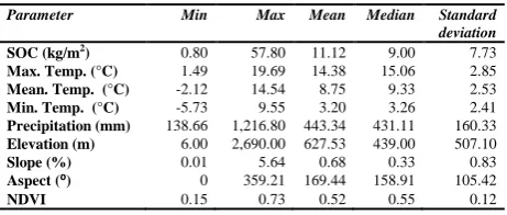
The statistical description of SOC and environmental determinants is summarized in Table 1. In Canadian forest areas, SOC stock ranges from 0.8 kg/m2 to 57.8 kg/m2. Compared to the maximum SOC stock (57.8 kg/m2), the mean (11.12 kg/m2) and median (9 kg/m2) values are relatively small. The standard deviation of SOC stock was 7.73 kg/m2, suggesting that only a small number of samples have very high SOC stock. Some soil samples were collected from the areas with very low vegetation biomass (NDVI = 0.15), such as mountainous areas and the forest-tundra zone. Moreover, all soil samples were collected from low-relief areas, with the maximum percent of slope of 5.64 % (equals to 3.23 degrees).
Table 1. Descriptive statistics of SOC stock and ecological variables within the study area (n = 1,317)
Parameter Min Max Mean Median Standard
deviation
SOC (kg/m2) 0.80 57.80 11.12 9.00 7.73
Max. Temp. (°C) 1.49 19.69 14.38 15.06 2.85
Mean. Temp. (°C) -2.12 14.54 8.75 9.33 2.53
Min. Temp. (°C) -5.73 9.55 3.20 3.26 2.41
Precipitation (mm) 138.66 1,216.80 443.34 431.11 160.33
Elevation (m) 6.00 2,690.00 627.53 439.00 507.10
Slope (%) 0.01 5.64 0.68 0.33 0.83
Aspect (⁰) 0 359.21 169.44 158.91 105.42
NDVI 0.15 0.73 0.52 0.55 0.12
Calculated from the historical soil profiles (Figure 4), B.C. coastal areas (Pacific Cordilleran eco-region) holds the maximum SOC stock of about 28 kg/m2. In the northern woodlands (Subarctic Cordilleran and Subarctic eco-regions), SOC stock is relatively high ranging from 12 kg/m2 to 17 kg/m2. The lowest mean SOC stock of about 9.7 kg/m2 was surprisingly observed in the largest Boreal eco-region.
Figure 4. Mean SOC stocks (1961-1991) of each Canadian forest eco-region
3.2 Spatial Data Analysis of Canadian Forest SOC
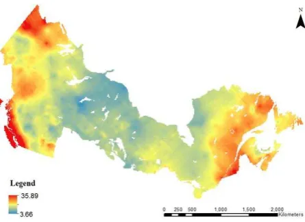
A fitted semi-variogram of SOC levels in the study area is shown in Figure 5 with a nugget effect of 0.211 and total sill of 0.391. The high nugget-to-sill ratio of 54% indicates that strong local-scale variations exist. A spatially continuous SOC distribution map was estimated using Ordinary Kriging (Figure 6). A west-to-central gradient of decreasing SOC stock and an increasing trend from central to eastern regions are observed. Forest SOC stock ranges from 3.66 kg/m2 to 35.89 kg/m2, which is a lower range than shown in Table 1. The leave-one-out cross validation approach resulted in a Pearson correlation coefficient of 0.76, indicating that the interpolated SOC values are in relatively good agreement with the measured SOC stocks.
Figure 5. Semi-variogram model of Canadian forest SOC distribution using Ordinary Kriging based on 1,317 samples
collected from the Canada Forest Service
Figure 6. 10 km gridded SOC data (before 1991) for Canadian forest areas based on Ordinary Kriging of 1,317 soil samples
collected from the Canada Forest Service
3.3 Spatial Soil-Environment Modelling
3.3.1 Global Spatial Autocorrelation: The optimal neighbourhood-sizes at which ecological activities were believed to promote the most intensive cluster-pattern were measured based on Incremental Spatial Autocorrelation analysis (Table 2). At the national scale, the first peak Z-score occurred at a distance of about 313,805 m.
Table 2. Optimal distance for spatial analysis
Eco-region Samples Standard Deviation
Outliers Average Nearest Neighbor (m)
First Peak Z-Score Distance (m)
Entire study area
1,317 22,678.25 53 16,392.04 313,805.45
Subarctic 129 38,757.55 5 33,741.42 148,467.05
Boreal 649 22,504.70 21 18,371.85 260,811.32
Cool Temperate
86 21,150.86 6 17,706.42 114,605.65
Cordilleran 306 21,076.25 15 13,633.76 72,983.24
Interior Cordilleran
71 14,473.06 4 10,810.77 57,580.51
Pacific Cordilleran
62 23,451.71 1 11,746.60 94,840.38
As shown in Table 3, the global Moran’s I of SOC at the national scale is about 0.289, which is relatively low yet statistically significant (p < 0.01). Positive global spatial autocorrelation indicates that spatial clusters of SOC may be found across the study area, with similar values clustering close together. To explore how SOC is distributed in different climatic zones, the global Moran’s I index of each eco-region were calculated with a maximum Moran’s I (0.391) observed in the Subarctic eco-region, while the minimum Moran’s I (0.069) was the Cordilleran eco-region. This suggests that although spatial dependence in SOC samples in the Cordilleran eco-region is significant, it is still nevertheless very weak.
Table 3. Global Moran’s I values for each eco-region
Eco-region Moran’s I value
All Eco-regions (entire study area) 0.289
Subarctic 0.391
Boreal 0.154
Cool Temperate 0.267
Cordilleran 0.069
Interior Cordilleran 0.281
Pacific Cordilleran 0.193
3.3.2 Local Spatial Autocorrelation: A local spatial autocorrelation (LISA) map of SOC distribution at the national scale is shown in Figure 7. It was observed that the SOC outliers were distributed throughout HH and LL clusters across the entire study. This likely contributes to the strong nugget effect that was previously observed (Figure 5). Due to local variations, any sample of relatively higher SOC stock (e.g., perhaps due to poor drainage) is considered to be an outlier within a LL cluster. In addition, multiple HH clusters are identified, including along the southwest coast. This finding is consistent with descriptive statistics, confirming that the B.C. forest coastal areas are rich in terms of SOC stocks.
A small HH cluster was also observed in the south-east of Québec forests, where the growing season is warmer and longer. Another significant HH cluster is on the border of Yukon and Northwest Territories, corresponding to the Peel Watershed. When comparing the location of HH clusters to a map of forest age distribution, it was found that all three HH clusters are located in old-growth forest areas (green-blue areas in Figure 8). The International Archives of the Photogrammetry, Remote Sensing and Spatial Information Sciences, Volume XL-2, 2014
Figure 7. Local spatial autocorrelation (LISA) cluster map of SOC distribution at the national scale
Most SOC LL clusters were located in central forest ecosystems, suggesting that soils in these regions have comparatively low carbon stock compared to the rest of the study area. The LL clusters encompass the Western Boreal eco-region, which has a drier and warmer climate compared to other eco-region classifications and consists of forest groups of a majority within the range of 10 years to 30 years (Figure 8). All of these attributes potentially explain why lower SOC levels are observed in this region.
Figure 8. Distribution map of forest age (1973 to 1998)
The LISA map SOC distribution in the Subarctic eco-region is shown in Figure 9. Soil samples with higher organic carbon stock (highlighted by a red ellipse) are mainly clustered in Peel Plateau and Peel Plain region. Soils in this area are usually cold and wet (likely affected by snowmelt), and thus accumulate a considerable amount of organic matter, as highlighted by a HH cluster. Another small HH cluster occurs along the east coast, mainly located in Melville Lake estuary (Newfoundland and Labrador). This area is also considered to be an area of interest where ongoing soil organic matter research is being undertaken (e.g., the Earth Science Laboratory of Memorial University). A LL cluster was also observed in central Quebec, where there is little vegetation biomass. This may also play a role in influencing SOC distribution.
Figure 9. LISA cluster map of SOC distribution in the Subarctic eco-region with the Peel Watershed area labelled
For the Boreal eco-region, as shown in Figure 10, LL patterns were mainly observed in western regions (e.g. Alberta, Saskatchewan, and Manitoba) and HH patterns in eastern regions. This spatial pattern is quite consistent with the precipitation regime and the forest age distribution characteristic of this region. Partly caused by the strong local variations in SOC stock, the distribution of LL clusters was not homogeneous with many HL outliers also prevalent. Western Boreal areas experience a mixed forest age distribution, thus different amounts of litterfall potentially result in variations in SOC stocks. Differences in other terrain attributes (e.g. drainage capacity) may also partly account for SOC variation.
Figure 10. LISA cluster map of SOC levels in Boreal eco-region
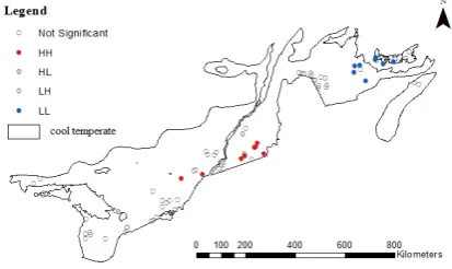
The SOC distribution pattern in the Cool Temperate eco-region is mainly characterized by a single HH cluster and LL cluster (Figure 11). Soil samples with high organic-carbon stock are clustered in the St. Lawrence watershed, which receives the highest level of precipitation. The LL cluster is observed around Prince Edward Island (PEI).
Figure 11. LISA map of Cool Temperate eco-region SOC levels The International Archives of the Photogrammetry, Remote Sensing and Spatial Information Sciences, Volume XL-2, 2014
Figure 12. LISA maps of SOC levels in Interior Cordilleran eco-region (left) and Pacific Cordilleran eco-region (right)
The cluster patterns of the Interior Cordilleran and Pacific Cordilleran eco-regions are not apparent. A small LL cluster is observed in low-lying areas (about 850 m elevation) of the Interior Plateau (Figure 12), where the climate is dry and vegetation does not effectively contribute to SOC accumulation. Although the overall SOC stock is high in the Pacific Cordilleran eco-region, a LL cluster is observed in the northern region (Figure 12). This is likely caused by insufficient rainfall input and less vegetation biomass. Another LL cluster is identified in the Lower Fraser Basin in southern B.C. Province.
3.3.3 Spatial Soil-Environment Modelling: From the spatial autocorrelation results presented in Section 3.3.2, significant spatial dependency in SOC distribution at the national scale was noted. Any statistically significant Moran’s I value suggests that it is necessary to take spatial effects into consideration. Before specifying a spatial regression model, a traditional OLS model is tested. The models are based on six independent variables: precipitation, temperature, NDVI, elevation, slope, and aspect. The selection of a spatial regression model specification is determined based on the Lagrange Multiplier diagnostic. A statistically significant LM-lag test suggests the inclusion of a spatially LM-lagged dependent variable, while a statistically significant LM-error test suggests adding an autocorrelated error term. When both tests are statistically significant, robust versions are tested for model specification.
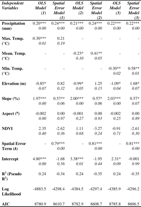
Table 4 shows the results of the initial estimation of three OLS models. Regression model (1), (2), and (3) differ in terms of the type of temperature readings included in the model specification, based on maximum, mean, and minimum temperature. For the three estimated OLS models, the R2 values were approximately 0.24, indicating that about 24% of variation in SOC distribution was explained by the initial OLS models. With the exception of NDVI and aspect, all other four independent variables were statistically significant at a 10% level. Compared to other independent variables, precipitation (p = 0.000) was shown to have the most significant influence on SOC distribution at the national scale.
To evaluate the performance of three OLS models, the strength of residual spatial autocorrelation was measured based on the Moran’s I test statistic. As shown in Table 5, all three Moran’s I tests were positive and highly significant (p < 0.01), indicating that spatial dependency is present in the regression residuals. Thus, spatial regression models were tested to take spatial information into consideration. The results of Lagrange
Multiplier tests are shown in Table 5. Since both standard LM-lag and LM-error tests were highly significant (p = 0.001), robust versions were tested for model specification. The robust LM-error tests (p = 0.000) were slightly more significant than the robust LM-lag tests (p = 0.001). Therefore, a spatial error regression model specification was selected.
Table 4. OLS and spatial error regression models of relationships between SOC (dependent variable) and environmental factors (independent variables) (n=1317). Models (1), (2), and (3) include maximum, mean, and minimum
temperature as one of the independent variables, respectively.
Independent
Table 5. Lagrange Multiplier diagnostic tests for SOC-environment relationships. Model (1), (2), and (3) include maximum, mean, and minimum temperature, respectively.
Dependence Test Value
Model (1) Model (2) Model (3)
A spatial error model specification suggests that cluster patterns in Canadian forest SOC distribution are likely due to the omission of other spatially autocorrelated variables potentially influencing SOC distribution, such as soil pH and nitrogen content. These factors were not included in this analysis due to data availability. Compared to initial OLS models (Table 4), general improvements in model fit (e.g., lower AIC values and higher log likelihood values) are observed. Precipitation (p = 0.000) was the most significant environmental determinant influencing SOC. The spatial error term (λ) was also statistically significant (p = 0.000), further supporting the notion that important unobservable or unmeasurable variables are missing from the model specification. Initial estimation of spatial error models suggested that aspect of slope and NDVI had a weaker relationship with SOC distribution. Compared to maximum and mean temperature (p = 0.192, p = 0.046), the minimum temperature regime (p = 0.011) had a more significant relationship with SOC distribution in Canadian forest areas.
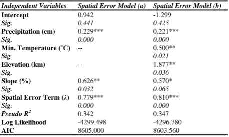
In order to improve the performance of spatial error models, independent variables that were less significant (p > 0.1) were removed from the model specification. As shown in Table 6, the re-estimated spatial error model (a) includes two independent variables, namely precipitation and slope, while model (b) also includes elevation and minimum temperature. Comparing the two models, the AIC values remained almost the same, suggesting minimal improvement in the model goodness of fit. Compared to the initial spatial error model (3) (Table 5), an increase in the significance of independent variables resulted in the re-estimated model (b) (p < 0.05). This finding suggests that model (b) is the best model fit. All ecological variables and the error term were positively related to the SOC distribution, while precipitation proved to be the most important variable (p = 0.000). Therefore, we conclude that four dominant ecological variables influence SOC distribution at the national scale: precipitation, minimum temperature, elevation, and slope.
Table 6. Re-estimated spatial error models of relationships between SOC (dependent variable) and environmental factors
(independent variables) (n=1,317). Model (a) includes two independent variables of precipitation and slope. Model (b) also
includes minimum temperature and elevation.
Independent Variables Spatial Error Model (a) Spatial Error Model (b)
Intercept
Sig.
0.942
0.441
-1.299
0.425
Precipitation (cm)
Sig.
0.229***
0.000
0.221***
0.000
Min. Temperature (˚C)
Sig
-- 0.500**
0.021
Elevation (km)
Sig.
-- 1.877**
0.036
Slope (%)
Sig.
0.626**
0.032
0.570*
0.065
Spatial Error Term (λ)
Sig.
0.779***
0.000
0.810***
0.000
Pseudo R2 0.342 0.347
Log Likelihood -4299.498 -4296.780
AIC 8605.000 8603.560
3.4 Predictive SOC Distribution Map
At the national scale, spatial regression results indicated four ecological variables that have dominant influence on Canadian forest SOC distribution, namely precipitation, elevation, minimum temperature, and slope. Accordingly, a predictive SOC distribution map in the period 1961-1991 was generated from the three-step procedure previously described in Section 2.3.
Figure 13. (a) Predictive SOC distribution (1961-1991) estimated from spatial error model parameters. (b) Interpolated SOC distribution (1961-1991) using Ordinary Kriging based on CFS SOC data. For each map, the SOC stock is standardized from zero to one by dividing the difference between raw SOC stock and the minimum value by the range of raw SOC stock.
Since it is difficult to obtain absolute SOC stock from the modelled SOC distribution map based on four ecological variables, the modelled SOC stock was standardized to a range of zero to one for mapping or visualizing the forest SOC distribution gradient at a national scale. In order to make the modelled SOC distribution map comparable with the interpolated SOC map, the latter was also standardized to a range of zero to one. In this way, it was possible to examine the differences in spatial patterns between the modelled and interpolated SOC distribution maps. Figure 13 shows the final predictive SOC distribution map estimated by spatial error model parameters.
Figure 14. Spatial distribution of differences between the predictive SOC stock estimated from spatial error model parameters and interpolated SOC stock using Ordinary Kriging.
An image differencing method involved subtracting the interpolated SOC map from the previous predictive SOC map (Figure 14). It was found that general trends in SOC distribution were captured by the four dominant ecological variables. In general, SOC estimates in B.C. coastal areas were in high The International Archives of the Photogrammetry, Remote Sensing and Spatial Information Sciences, Volume XL-2, 2014
agreement, since differences were close to zero. However, larger differences in SOC estimates were observed in the Subarctic Cordilleran eco-region (Yukon Territory), southern Ontario, and Prince Edward Island. It should be noted that the legend values shown do not have absolute meaning, since they are calculated from pseudo SOC levels.
4. DISCUSSION & CONCLUSIONS
According to spatial autocorrelation analysis results, the eco-region framework proved to be a suitable classification scheme for SOC distribution patterns in Canada. Multiple HH SOC clusters were found in east and west coasts, which typically have a humid climate. LL clusters of low SOC levels were mainly concentrated in central continental regions, such as the Great Plains, which is characterized as arid or semi-arid. In B.C. mountainous areas, the global Moran’s I (0.069) suggests that local variations in SOC distribution exist, which could be attributed to complex geographic conditions and topography. Ehrlich et al. (1977) found that high soil clay content variability in B.C. mountainous areas were due to sediment movement and erosion processes, which may contribute to the weak spatial autocorrelation observed in this area.
Observed SOC spatial patterns also closely correspond to forest age distribution. According to Chen et al. (2003), forests in the B.C. coast and east Quebec are generally more than 100-year old with few disturbances detected, whereas young forests (between 10- to 40-years old) are mainly in western Boreal areas. Such regrowth forests are largely from fire disturbance and human inference, providing less carbon inputs into soils, leading to poor regional SOC sequestration ability. Consequently, findings from this study support the importance of protecting old-growth forests for SOC management.
Our assessment of relationships between SOC and environmental factors revealed a positive SOC-precipitation association. Sufficient rainfall supply maintains good water-saturation in soils, which tends to limit SOC decomposition rates. In this study, minimum temperature proved to have a significant and positive effect on SOC distribution. Recalling that SOC stock is the difference between organic-carbon inputs and carbon decomposition, any changes in the two processes will alter SOC stock. In mid- and high-latitude forest ecosystems, increasing minimum temperatures tend to result in a longer growing season. Thus, we conclude that although SOC decomposition rates tend to accelerate with increasing temperatures in forest areas, the amount of carbon loss is offset by increasing vegetation biomass and litterfall accumulation.
Moreover, the highly significant spatial error term in our estimated model, suggested that other important ecological factors may be excluded from this analysis. These could be immeasurable and unobservable factors, which would likely partly account for the variation in SOC distribution. This affirms that regional-scale interactions between SOC and its surroundings are quite complex to model. Many researchers have suggested that there is a lack of research into quantifying SOC distribution and modelling SOC-environment relationships (Galbraith et al., 2003). Thus, the effects of ecological factors on the Canadian forest SOC distribution are potentially underrepresented. Although using a spatial error model partly moderates the effects of omitted variables, the low pseudo R2 of 0.347 indicated that 65.3% of variation in SOC distribution pattern remains unexplained.
Finally, potentially missing independent variables ultimately limit the performance of regression models. As previously discussed, topographic factors such as forest age, soil pH, nitrogen content, and other soil properties were not considered due to data availability. With increasing data availability and improved data quality, the relationships between SOC and ecological variables are becoming better described. This information will, in turn, provide valuable information to better inform SOC management and land use practices.
REFERENCES
Anselin, L., 1988. Lagrange multiplier test diagnostics for spatial dependence and spatial heterogeneity. Geographical analysis, 20(1), pp. 1-17.
Anselin, L., 2005. Exploring spatial data with GeoDa: A workbook. Spatial Analysis Laboratory, IL, USA.
Buringh, P., 1984. Organic carbon in soils of the world. The Role of Terrestrial Vegetation in the Global Carbon Cycle. Measurement by Remote Sensing, Vol. SCOPE, 23.
Chen, J.M., Ju, W., Cihlar, J., Price, D., Liu, J., Chen, W., Pan, J., Black, A., Barr, A., 2003. Spatial distribution of carbon sources and sinks in Canada forests. Tellus, 55(2), pp. 622-641.
Ehrlich, W.A., Cann, D.B., Day, J.H., Marshall, I.B., 1977. Soils of Canada, Department of Agriculture, Vol. 1, pp. 73-77. ESRI, 2013. Modelling spatial relationships. http://resources.arcgis.com/en/help/main/10.1/index.html#/Mod eling_spatial_relationships/005p00000005000000/ (5 May 2014).
Galbraith, J.M., Kleinman, P.J.A., Bryant, R.B., 2003. Sources of uncertainty affecting soil organic carbon estimates in northern New York. Soil Science Society of America Journal, 67(4), pp. 1206-1212.
Lee, P., Hanneman, M., Gysbers, J., Cheng, R., 2010. Atlas of key ecological areas within Canada’s intact forest landscapes. Global Forest Watch Canada, Edmonton, Canada. 10th Anniversary Publication, No. 4.
Luyssaert, S., Schulze, E.D., Bӧrner, A., Knohl, A., Hessenmӧller, D., Law, B.E., Grace, J., 2008. Old-growth forests as global carbon sinks. Nature, 455(7210), pp. 213-215.
MacDonald, G.N., Gajewski, K., 1992. The northern treeline of Canada. In: Geographical Snapshots of North America: Commemorating the 27th Congress of the International Geographical Union and Assembly, pp. 34-37.
Mishra, U., Lai, R., Liu, D., Van Meirvenne, M., 2010. Predicting the spatial variation of the soil organic carbon pool at a regional scale. Soil Science Society of America Journal, 74(3), pp. 906-914.
Shakiba, A., Matkan, A., 2005. Sensitivity of global soil carbon to different climate change scenarios. Environmental Sciences, 9, pp. 13-24.
Tewksbury, C.E., Van Miegroet, H., 2007. Soil organic carbon dynamics along a climatic gradient in a southern Appalachian spruce-fir forest. Canadian Journal of Forest Research, 37(7), pp. 1161-1172.