www.elsevier.com / locate / livprodsci
Random regressions to model phenotypic variation in monthly
weights of Australian beef cows
,1
*
Karin Meyer
Animal Genetics and Breeding Unit, University of New England, Armidale NSW 2351, Australia
Received 7 July 1999; received in revised form 1 December 1999; accepted 1 December 1999
Abstract
Weights of beef cows recorded on a monthly basis were analysed using a random regression model. Data originated from a selection experiment in Western Australia, involving two herds of about 300 cows, Polled Herefords and a four breed synthetic, the so-called Wokalups. Weights were subject to large seasonal effects. Short mating periods and thus tight calving seasons led to substantial confounding between age and season at weighing. Records between 19 and 84 months were considered, up to 62 per cow, yielding 27 728 and 29 033 records for 922 and 1020 cows, respectively. Only phenotypic random regressions for animal effects, ignoring relationships, were considered. Covariances between regression coefficients and error variances were estimated by restricted maximum likelihood. A variety of models, involving random regressions on orthogonal polynomials of age, on segmented polynomials and on sine and cosine functions and different assumptions about the structure of error variances, were considered. Analyses identified a distinct cyclic, seasonal pattern of variation, both between animals and for temporary environmental effects. This could only partially be attributed to scale effects. Orthogonal polynomials proved well capable of modelling such sinuousity but required a high order of fit and thus a large number of parameters. Alternative curves utilising the known periodicity (12 months) provided more parsimonious parameterisations. Due to the high degree of confounding between age and season of recording their contributions to the total variance could
not be separated. 2000 Elsevier Science B.V. All rights reserved.
Keywords: Random regression; Growth curve; Modelling; Mature weights; Beef cattle
1. Introduction 1998c). In particular, RR models accommodate
‘repeated’ records for traits which change, gradually Random regression (RR) models and the resulting and continually, over time, and do not require covariance functions (CF) have recently been recog- stringent assumptions about constancy of variances nised as ideally suited to the analysis of longitudinal and correlations. RR models for the analysis of data data in animal breeding and the description of the from animal breeding schemes have first been pro-resulting covariance structure (Hill, 1998; Meyer, posed to model test day production records of dairy cows (Schaeffer and Dekkers, 1994). Applications so far have concentrated in this area, e.g. Jamrozik and
*Tel.: 161-26-773-3331; fax:161-26-773-3266.
Schaeffer (1997), Jamrozik et al. (1997), Kettunen et
E-mail address: [email protected] (K. Meyer)
1
A joint unit with NSW Agriculture. al. (1998), Van der Werf et al. (1998), Tijani et al.
(1999), Rekaya et al. (1999), Veerkamp and Thomp- growth and its variation parsimoniously. While we son (1999) and Brotherstone et al. (2000). are ultimately interested in a genetic analysis, as a Other traits of prime interest in livestock pro- first step, only phenotypic animal effects and growth duction which are measured over time and for which curves are considered.
a simple repeatability model, assuming constant variances and correlations, clearly does not hold are
those related to growth of animals. In standard 2. Material and methods
analyses, this has so far generally been taken into
account by treating records in different age intervals 2.1. Data as different traits. For example, genetic evaluation of
beef cattle often considers four different growth Data consisted of weights of cows collected as traits, namely birth, weaning, yearling and final part of a selection experiment at the Wokalup weights, with the latter three defined as weights agricultural research station, located in the South of taken, say, from 80 to 300 days, 301 to 500 days and Western Australia, approximately 140 kilometers 501 to 700 days of age, respectively. Clearly, this is South of Perth. Details of the experiment and somewhat arbitrary and a RR / CF model using each management strategies at the research station have record at the age it was taken would be more been described by Meyer et al. (1993). The experi-appropriate. Indeed, Kirkpatrick et al. (1990) de- ment comprised two herds of about 300 cows each, a veloped their ‘‘infinite-dimensional’’, CF model with purebred Polled Hereford (PH) herd and a herd of a the analysis of growth traits in mind. four-breed synthetic, formed by mating Charolais 3
RR models have been used for some time in the Brahman bulls to Friesian 3 Angus or Friesian 3
analysis of human growth curve data. Laird and Hereford cows, the so-called ‘Wokalups’ (WOK). Ware (1982) outlined a RR mixed model for longi- Selection for improved preweaning growth rate tudinal data which comprised both growth curve began in 1978.
models and repeatability models as special cases. In Management of the herds was characterised by animal breeding, selected growth curves, such as short mating periods of seven to eight weeks, Gompertz or Richards functions, have commonly resulting in the bulk of calvings in April and May been fitted to growth records. To date, however, this each year. Weaning took place in December. Except has generally been done independently to the estima- during the calving season, cows and calves were tion of fixed and random effects, i.e. not within a weighed at monthly intervals throughout the experi-linear mixed model framework. Anderson and ment. While the research station has reasonable Pedersen (1996) showed how RR can be employed rainfalls (annual average 979 mm), the climate is in modelling growth curves of pigs on a phenotypic Mediterranean with high levels of precipitation dur-level. Meyer (1999) presented an application to ing winter and an annual summer drought, from mature cow weight records in beef cattle, contrasting November to April the following year. This resulted analyses fitting RR coefficients for phenotypic ani- in strong seasonal variation in pasture availability mal effects only to those attempting to partition and, consequently, weight of cows.
prob-lems associated with small numbers per age and as the independent covariable or ‘meta-meter’. This contemporary group encountered in earlier analyses involved fitting a set of regression coefficients on age considering January weights up to 119 months or functions thereof for each animal as random (Meyer, 1999). Similarly, small numbers of records effects. Different assumptions on the shape of taken during April and May were excluded from the growth curves could be accommodated by choosing analysis. This yielded 27 728 records for 922 PH the functions of age appropriately. Only regression cows and 29 033 records for 1020 WOK cows, coefficients pertaining to phenotypic animal effects respectively, and a maximum of 62 ‘repeated’ re- were considered, i.e. no attempt was made to sepa-cords per cow. Weights ranged from 193 to 836 kg rate overall animal effects into their genetic and for PH and 226 to 946 kg for WOK. permanent environmental components, and relation-ships between animals were ignored. Fixed effects in 2.2. Analyses the model of analysis were CG, defined as above, and a fixed, cubic regression on orthogonal polyno-2.2.1. Preliminary analyses mials of age to model population age trends. Analy-Preliminary analyses were carried out to character- ses were carried out using a combination of average ise the pattern of variation in the data. Firstly, information and derivative-free REML algorithms as variances within age classes were examined for outlined by Meyer (1998b) and implemented in records adjusted for contemporary group (CG) ef- program DXMRR (Meyer, 1998a).
fects, defined as paddock-year-week of weighing Analyses yielded estimates of covariances among subclasses, both on the original scale and for data random regression coefficients and estimates of transformed to logarithmic scale. This used estimates variances due to temporary environmental variances, of CG effects obtained from simple least-squares so-called measurement error variances. From these, analyses ignoring animals but fitting a fixed regres- estimates of covariance functions and of variances sion on orthogonal polynomials of age. and covariances among ages in the data were ob-‘Standard’ univariate REML analyses considering tained. A variety of models involving different records for individual ages were carried out to assess regression curves and assumptions on the distribution the proportion of variation due to animals. Analyses of measurement errors were fitted, more than 100 in fitted phenotypic animal effects as random effects total. Due to computational limitations, most models and ignored any relationships between animals. Thus were examined for PH only, fitting only selected repeated records per animal were required to separate cases for WOK. The majority of analyses were variances due to animals and temporary environmen- carried out for weights as measured. In addition, a tal effects. Hence analyses for the i-th age (i5 small number of analyses considered records trans-19,84) considered ages i21, i and i11, i.e. in- formed to logarithmic scale.
volved records from 18 to 85 months of age, and Models were compared using likelihood ratio tests included any records taken during the calving (LRT) and by comparing estimated standard devia-season. Fixed effects fitted in these analyses were tions for the ages in the data. When testing whether CG and age (three classes). In addition, similar additional regression coefficients should be fitted, i.e. analyses were carried out considering weights re- whether the (co)variances for the additional coeffi-corded in a particular month only. The model for the cients were different from zero, hypotheses involved latter analyses again fitted animals as random and points at the boundary of the parameter space and, as CG as fixed effects but accounted for age as record- shown by Stram and Lee (1994), conventional LRT ing by fitting it as a linear and quadratic covariable. tend to be too conservative. Where applicable, this All univariate analyses were carried out using pro- was counteracted by doubling the error probability gram ASREML (Gilmour et al., 1999). when conducting LRTs.
Orthogonal polynomials. The first set of analyses
z
(LP), and in the following ‘‘LPk’’ denotes a model
2
range, a , the r-th polynomials is given as (e.g.j
Abramowitz and Stegun (1965))
the first term is a scalar, i.e. a polynomial of order k z
involves powers of age up to k21. 1
O
bi( 31r)a 1 eir ij (5)r51
This gives the model for the j-th weight yij
*
recorded for animal i at age aij (aij on the stan- with dardised scale) as
Knots were chosen after inspection of results from with F representing the fixed effects pertaining toij the preliminary, univariate analyses and RR analyses
y ,ij bir denoting the set of k random regression fitting LPs. Placing knots at the lowest weights (Fig. coefficients for animal i (the ‘animal effects’), andeij 1) and standard deviations and dividing ages into 12 the corresponding residual error. months segments with the first knot at 25 months of
Segmented polynomials. Secondly, models in- age resulted in 5 knots, at 25, 37, 49, 61 and 73 volving RR on segmented quadratic (SQ) or cubic months, respectively. This resulted in segmented (SC) polynomial functions were examined. Such quadratic and cubic polynomials with 8 and 9 functions, also called piecewise polynomials or, parameters, denoted by SQ8 and SC9. Reducing sometimes, grafted polynomials (Fuller, 1969), are segments to 6 months intervals gave 10 knots (at 25, the equivalent to spline functions used widely in 31, 37, 43, 49, 55, 61, 67, 67, 73 and 79 months) and non-parametric regression analyses. They are linear models SQ13 and SC14 with 13 and 14 regression in the parameters to be estimated and thus suitable coefficients, respectively. In addition, quadratic poly-for RR model analyses in a linear mixed model nomials with knots at 20,32, . . . ,80 months (z56), framework. As the name says, segmented polyno- and knots at 20,26, . . . ,80 months (z511), yielding mials allow approximation of a function by different models SQ9 and SQ14 respectively, were examined. polynomials in individual segments. Points at which Procedures to estimate the position of knots simul-segments join are commonly referred to as nodes or taneously with the regression coefficients are avail-knots. Segments are required to be continuous and able (e.g. Gallant and Fuller (1973)). This should have continuous first and, if they exist, non-zero also be feasible in a REML framework of estimation. higher order derivatives. Together with the assump- However, this was not investigated.
tion that segments are of the same form, this reduces Fourier series approximation. Preliminary
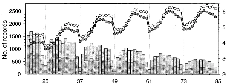
Fig. 1. Numbers of records (dark grey: Polled Hereford, light grey: Wokalups) and mean weights (d: Polled Hereford,s: Wokalup) for ages in the data.
period function F(t) with period T can be represented sets of RR coefficients were independent or allowing by an infinite series of form for covariances between them. Let ‘‘Ff ’’ denote the Fourier part of (8) with f variables. Using ‘1’ to
`
a0
symbolise that two separate, uncorrelated sets of RR
]
F(t)5 2 1
O
a cos(rr vt)1b sin(rr vt) (7)r51 coefficients were fitted, ‘‘Pp1Ff ’’ then denotes a
model with a total of p1f coefficients and p( p11) / with v 52P/T, and a and b the so-called Fourieri i
21f( f11) / 2 covariances between RR coefficients coefficients, which are given by various integrals of
to be estimated. Conversely, ‘‘PpFf ’’ (no ‘1’) is the
F(t) over a single period T. The coefficients have an
corresponding model allowing for covariances be-interpretation in their own right, representing
fre-tween the two types of regression coefficients, quency components of the function.
resulting in ( p1f )( p1f11) / 2 parameters due to For RR analyses, T was assumed to be 12 months,
RR. For instance, LP121F4 describes a model i.e v¯0.5235. Approximations involving one, two
fitting LP to order k512 together with a Fourier and three sets of sine and cosine functions, i.e. 2, 4
series approximation involving 2 sine and 2 cosine and 6 RR coefficients for each animal, were
consid-functions. Since the two sets of RR coefficients are ered. The expansion given by (7) is appropriate for a
assumed uncorrelated, the total number of covar-function with a level baseline. To account for age
iances between RR coefficients is 12313 / 2143
trends, Fourier series regressions were thus fitted
5 / 2588. LP12F4 is the same model accounting for jointly with one of the polynomials described above,
non-zero covariances with 16317 / 25136 compo-i.e., in essence, substituting a polynomial in age for
nents to be estimated. the scalar term (a0/ 2) in (7). Let f denote the
Regression on second ‘meta-meter’. In addition,
number of regression coefficients for the Fourier
analyses were carried introducing a second indepen-series fitted, and ‘‘Pp’’ a polynomial (LP or SQ) with
dent, continuous variable, namely month of
record-p regression coefficients on functions of age g(a ).ij
ing (m ), and fitting an additional set of RR for each This gives the model of analysis ij
animal, regressing on month or functions thereof,
f / 2 p
h(m ). Covariances between RR on months and RRij
yij5Fij1
O
birg(a )ij 1O
bi( p12r21 )cos(rva )ij on age were assumed to be zero, and, as above, this r51 r51is denoted by ‘1’. Both orthogonal polynomials and
1bi( p12r)sin(rva )ij 1eij (8)
2, 6 and 10. With records for April and May not other ages from this estimate and the estimated included in the analysis, there were 10 different regression line. Orders of polynomial fit of 5, 7, . . . ,
2
months, i.e. the latter represented a full order fit. 17, 19 were examined. Finally,sei were assumed to Models including a regression on months are denoted change in a cyclic fashion over the year. Hence 12
2
as ‘‘Pp1M Qq’’ with ‘‘Pp’’ as above the polynomial] components were fitted, assuming se1 pertained to
2
of age with p coefficients, and ‘‘Qq’’ standing for the 25, 37, 49, 61 and 73 months of age, se2 to 26,
2
function involving q parameters which was used to 38, . . . , 74 months, . . . , se7 to 19, 31, . . . , 79
2
model month. For weight yij recorded at age aij in months, . . . , and se12 to 24, . . . , 84 months. This month m ,ij error structure is denoted as ‘‘E12C’’.
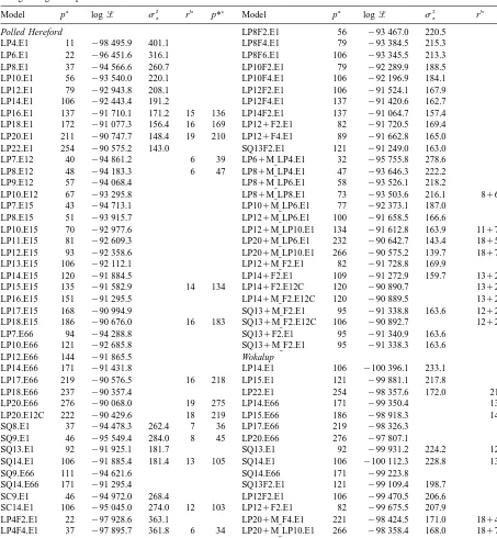
Table 1 summarises the random regression models
p q
examined and abbreviations used to describe them.
yij5Fij1
O
birg(a )ij 1O
bi( p1r)h(m )ij 1eij (9)r51 r51
For example, LP121M F2 is a model fitting a RR] 3. Results
on orthogonal polynomials of age to order k512
and a RR on the first set of sine and cosine functions 3.1. Characteristics of the data in a Fourier series, with 12313 / 21233 / 2581
covariances between RR coefficients. Means and numbers of records for the 66 ages in
Measurement error variances. All models in- the data are shown in Fig. 1. Low numbers of cluded a random error term,eij, representing tempor- records at 25, 37, . . . , 73 months reflect lack of ary environmental effects or so-called measurement recording of cow weights during the calving season. errors. These were assumed to be independently Mean weights for both breeds followed a distinct 12 distributed for all analyses. Several alternatives month cycle with an amplitude, i.e. difference be-regarding the number (m) of different measurement tween highest and lowest mean weights, of about
2
error variances (sei, i51, m) required to model 100 kg. WOK cows were larger than PH cows temporary variation in the data adequately were throughout, with differences tending to be bigger at investigated. Thus complete description of the the higher than at lower weights.
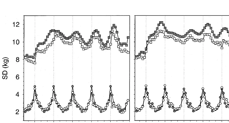
RR model used required augmenting the abbrevia- Corresponding standard deviations within age tions given above by a term ‘‘.Em’’. For example classes are depicted in Fig. 2 (left graph). Records LP20.E15 is a model fitting LP with k520 and 15 for WOK tended to be more variable than for PH.
2
individualsei. Firstly, variances were considered to Transforming records to logarithmic value substan-be homogeneous, i.e. m51, consistent with the tially reduced this difference, indicating that it was concept of a measurement error affecting all records mainly due to scale effects. Moreover, the trans-equally. Secondly, variances were allowed to be formation emphasized a cyclic pattern in variation at heterogeneous, changing with age. Fitting individual individual ages, again following cycle of about 12
2
sei for every six-month interval (i.e 19–24, . . . , months. Peaks for PH at 37, 49 and 61 months 79–84 months) yielded m512 components. Sub- represented ages with few records (c.f. Fig. 1) and
2
dividing the first and last interval so that separatesei could not be attributed to the same animals. They were fitted for the first (last) and second plus third were thus treated as random fluctuations. Adjusting (second-last plus third-last) age (i.e. 19, 20–21, 22– records for least-squares estimates of CG effects 24, 25–30, . . . , 73–78, 79–81, 82–83, 84 months) showed a similar pattern (Fig. 2, right graph), with increased the number to m515. Allowing for a differences in variances between ages particularly different variance for each age resulted in a model pronounced for WOK.
with m566 error variances to be estimated. Thirdly, With a short mating period and, consequently,
2
Table 1
Random regression models fitted
a
Abbreviation LPk SQ(31z) SC(41z) Ff M Pp] Em
Function Legendre Segmented Segmented Fourier Regression Error
Polynomial quadratic cubic approximation on month structure polynomial polynomial
Features Order k z knots z knots f/ 2 sine and Polynomial P m variance cosine functions with p parameters components
Equation (2) (3) (5) (8) (9)
Cases LP4 SQ8 SC9 F2 M LP4] .E1
LP6 SQ9 SC14 F4 M LP6] .E12
LP8 SQ13 F6 M LP10] .E15
LP10 SQ14 M F2] .E66
LP12 M F4] .E12C
LP14 LP16 LP18 LP20 LP22
a
Brackets for clarity here only.
Fig. 2. Standard deviations within age class for raw data (left graph) and records adjusted for fixed effects (right graph) for weights (in kg; circles) and weights transformed to logarithmic sale (log kg 3100; squares) for Polled Herefords (closed symbols) and Wokalups (open symbols).
Fig. 3. Numbers of records (bars) and mean weights (d) for individual months of recording (total number and average over both breeds, respectively).
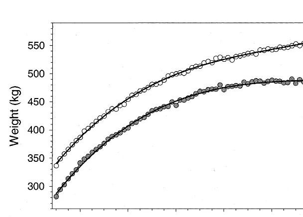
Fig. 4. Estimated population trajectory (fixed, quadratic regression on orthogonal polynomials of age) from least-squares analysis ignoring random effects together with means for ages of records adjusted for fixed effects except the regression on age, for Polled Herefords (d) and Wokalups (s).
fluctua-tions in variance. Hence the pattern of variation tween corresponding estimates of sP was as low as
2
shown in Fig. 2 (right graph) is what needed to be 0.064 kg with a maximum difference of 0.7 kg at 62 modelled in RR model analyses. months. Increasing k until log + ceased to increase
would have been desirable but was disregarded due 3.2. Random regression on orthogonal polynomials to the large number of parameters to be estimated
of age simultaneously, as large as 254 at k522, and the resulting computational requirements. Modelling Log likelihoods (log+) from RR analyses on the liveweight changes in lactating dairy cows using RR
original scale are summarised in Table 2, and on orthogonal polynomials, Koenen et al. (1999) corresponding values for data transformed to loga- also found that, based on LRTs, a high order of rithmic scale are given in Table 3. For models polynomial fit was required.
assuming homogeneous measurement error variances
2
(‘‘.E1’’), estimates of sei are given in addition. 3.3. Modelling measurement error variances
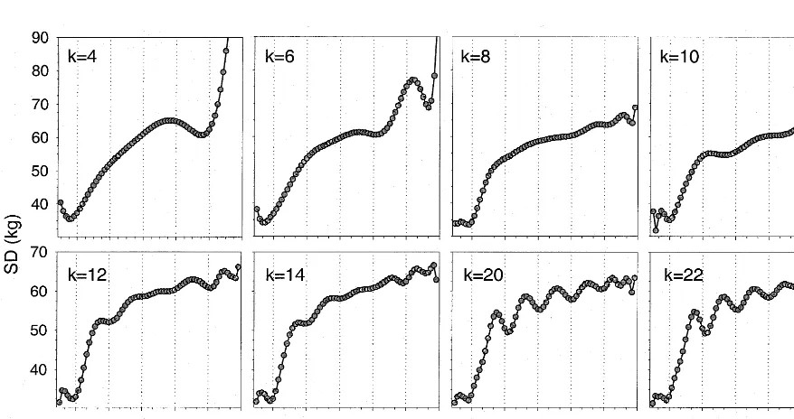
Which order of fit? Phenotypic standard
devia-tions for PH from analyses fitting RRs on orthogonal Similar patterns were observed for analyses fitting polynomials and a single measurement error variance multiple measurement error variances (Models (Models LPk.E1) are shown in Fig. 5, for orders of LPk.E12, LPk.E15 and LPk.E66). As illustrated in fit ranging from k54 to 22. For previous analyses of Fig. 6, log + increased with the order of fit at
January weights only, a cubic polynomial, i.e. k54, approximately the same rate for different assump-sufficed to model growth of cows from 19 to 118 tions about the variance structure of temporary months of age adequately (Meyer, 1999). Consider- environmental effects. Plotting log + against the
ing records throughout the year, however, this was number of parameters ( p) estimated shows that at
2
clearly inappropriate, with phenotypic standard de- low p a singlesei(m51) provided the best fit to the viations (sP) derived from the estimated CF increas- data since for constant p it allowed the highest k.
2
ing sharply for the last 12 ages in the data, reaching Conversely, individual sei (m566) were only ad-132.5 kg for 84 months. In contrast, the estimate of vantageous, at equal numbers of parameters fitted,
sP at 84 months from a univariate analysis was 52.8 for high orders of fit (k$17) and large numbers of
kg. parameters ( p.211).
Increasing k reduced the obvious upwards bias in Estimates of standard deviations from analyses estimates ofsP for the latest ages, i.e. the ages with fitting RR on LPs of age allowing for different the least records. An order of k512 was required numbers of measurement error variances are con-before estimates of sP for cows older than 6 years trasted in Fig. 7. While estimates of se differed settled around the 60 kg mark. For orders of fit larger substantially for m51, m515 and m566 and log than k512, the overall trend in estimates ofs over + increased markedly and significantly with
increas-P
time changed little. However, curves representingsP ing number of variance components fitted, there was exhibited more and more oscillations as k increased little difference in estimates of between animal (k516 and k518 not shown). As shown in Table 2, standard deviations for k$12. Differences in esti-likelihoods increased dramatically with increasing mates of sP (not shown) were then largely due to order of polynomial fit, accompanied by a steady differences in estimates ofse. Corresponding results
2
decline in the corresponding estimates of sei. have been reported by Olori et al. (1999), who found With large numbers of records per individual, all no significant differences in estimates of additive increases in k yielded significant improvements in genetic and permanent environmental variances of log +. Augmenting k from 20 to 22 added 43 test day records in dairy cows when fitting different
(co)variances among RR coefficients to be estimated, numbers of measurement error variances. Similarly, increasing log + by 172.5, while there was little Snyder et al. (1999) reported only minor differences
Table 2
2
Maximum log likelihood values (log+) for different analyses, together with estimates of the measurement error variance (se) for models fitting a single component
a 2 b c a 2 b c
Model p log+ se r p* Model p log+ se r p*
Polled Hereford LP8F2.E1 56 293 467.0 220.5
LP4.E1 11 298 495.9 401.1 LP8F4.E1 79 293 384.5 215.3
LP6.E1 22 296 451.6 316.1 LP8F6.E1 106 293 345.5 213.3
LP8.E1 37 294 566.6 260.7 LP10F2.E1 79 292 289.9 188.5
LP10.E1 56 293 540.0 220.1 LP10F4.E1 106 292 196.9 184.1 LP12.E1 79 292 943.8 208.1 LP12F2.E1 106 291 524.1 167.9 LP14.E1 106 292 443.4 191.2 LP12F4.E1 137 291 420.6 162.7 LP16.E1 137 291 710.1 171.2 15 136 LP14F2.E1 137 291 064.7 157.4 LP18.E1 172 291 077.3 156.4 16 169 LP121F2.E1 82 291 720.5 169.4 LP20.E1 211 290 747.7 148.4 19 210 LP121F4.E1 89 291 662.8 165.0 LP22.E1 254 290 575.2 143.0 SQ13F2.E1 121 291 249.0 163.0 LP7.E12 40 294 861.2 6 39 LP61M LP4.E1] 32 295 755.8 278.6
LP14.E66 171 291 431.8 LP14.E1 106 2100 396.1 233.1
LP17.E66 219 290 576.5 16 218 LP15.E1 121 299 881.1 217.8
LP18.E66 237 290 357.4 LP22.E1 254 298 357.6 172.0 21 253
LP20.E66 276 290 068.0 19 275 LP14.E66 171 299 350.4 13 170
LP20.E12C 222 290 429.6 18 219 LP15.E66 186 298 918.3 14 185
SQ8.E1 37 294 478.3 262.4 7 36 LP17.E66 219 298 326.3 SQ9.E1 46 295 549.4 284.0 8 45 LP20.E66 276 297 807.1
SQ13.E1 92 291 925.1 181.7 SQ13.E1 92 299 931.2 224.2 12 91
SQ14.E1 106 291 885.4 181.4 13 105 SQ14.E1 106 2100 112.3 228.8 13 105
SQ9.E66 111 294 621.6 SQ14.E66 171 299 223.8
SQ14.E66 171 291 295.4 SQ13F2.E1 121 299 109.4 198.7
SC9.E1 46 294 972.0 268.4 LP12F2.E1 106 299 470.5 206.6
SC14.E1 106 295 045.0 274.0 12 103 LP121F2.E1 82 299 675.5 207.9
Reduced rank of estimated covariance matrix; left blank if matrix was not constrained.
c
Table 3
Maximum log likelihood values (log+) for analyses of data transformed to logarithmic scale, together with estimates of the measurement
2
error variance (se) for models fitting a single component
a 2 b c a 2 b c
Model p log+ se r p* Model p log+ se r p*
Polled Hereford SQ131M F2.E1] 95 252 091.4 7.8
LP20.E1 211 250 379.0 6.9 SQ131M LP2.E12C] 106 251 395.7 10 100
LP20.E12C 222 249 814.9 Wokalup
LP61M LP6.E1] 43 254 788.4 12.5 LP20.E1 211 254 079.5 7.3 LP101M LP6.E1] 77 251 911.2 8.8 LP20.E12C 222 253 395.6
LP121M LP6.E1] 100 251 316.7 7.9 LP121M LP6.E1] 100 255 127.1 8.4 LP121M F2.E1] 82 251 427.4 8.1 LP121M F4.E1] 89 255 088.0 8.3 LP121M F4.E1] 89 251 313.0 7.9 SQ131M F2.E1] 95 256 164.4 8.3
a
Number of parameters (full rank).
b
Reduced rank of estimated covariance matrix; left blank if matrix was not constrained.
c
Number of parameters if reduced rank covariance matrix has been estimated.
Fig. 5. Estimates of phenotypic standard deviations for Polled Herefords, from analyses fitting random regressions on Legendre polynomials of order k54 to k522, assuming homogeneous measurement error variances.
described by a quadratic function in age. This parameters to be estimated in individual analyses, suggests that for a sufficient order of fit, i.e. an order thus making model comparisons easier.
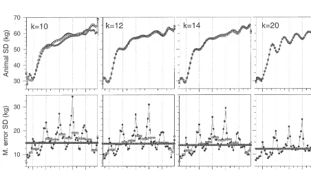
of fit which does not produce gross over- or under- Comparison with univariate estimates. When
2
Fig. 6. Maximum log likelihood for analyses of Polled Hereford data, fitting random regressions on Legendre polynomials of age, allowing for single (m51,j), grouped (m515,d) and individual (m566,m) measurement error variances.
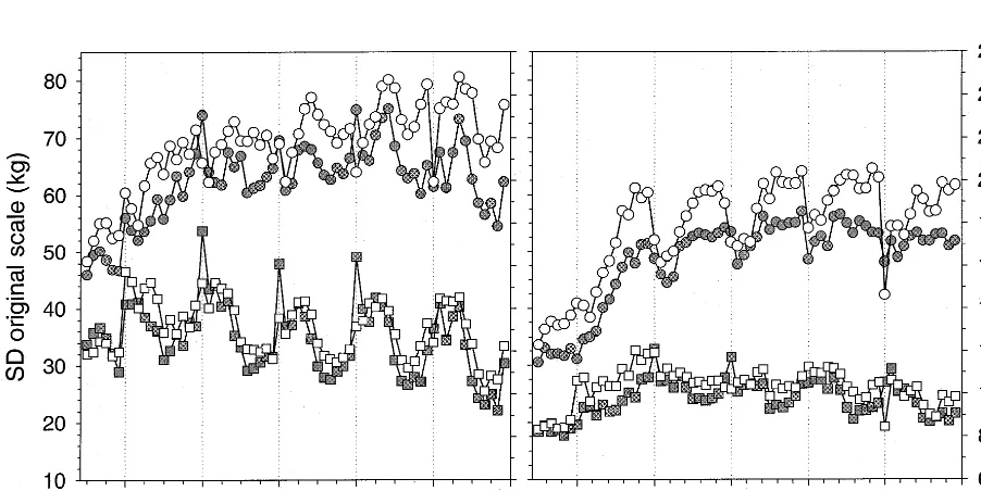
Fig. 8. Estimates of between animal (squares) and measurement error (circles) standard deviations (in kg) from univariate analyses (open symbols) and analyses fitting random regressions on Legendre polynomials of order k520 and allowing for separate measurement error variances for individual ages (m566) (closed symbols), for Polled Herefords (left) and Wokalups (right).
individual ages. Corresponding estimates of between models .E1 and .E12C were found for other RR animal components showed reasonable agreement for models for PH (LP141M F2, SQ13] 1M F2) and] earlier ages, in particular for WOK. Estimates from analyses on the logarithmic scale (Table 3). This both types of analyses followed a similar, cyclic suggests that the cyclic measurement error variances pattern, indicating that the RR model fitted modelled indeed represent a reasonable compromise between the existing variation in the data adequately. How- parsimony and adequateness of modelling temporary ever, values from RR analyses were consistently environmental variation. Conversely, it indicates that higher for later ages. Presumably, this reflected, in there were additional, age-specific and non-seasonal part at least, a reduction in variation between animals differences in variation which were only fully mod-due to culling: RR analyses incorporating records at elled by fitting individual measurement error vari-all ages are expected to account for this while their ances for all ages.
univariate counterparts are not. Regression line. Finally, it was attempted to
2
Cyclic measurement error variances. The pat- model changes inse over time through a polynomial tern in estimates of se observed above (Fig. 8) regression equation. This involved estimating a suggested that a model with 12 distinct components single measurement error variance at the mean age repeated cyclically (.E12C) might fit the temporary (0 on the standardised scale) and the coefficients of a
2
environmental variation in the data without increas- regression line to predict se at individual ages. A ing the number of parameters to be estimated similar approach, in retrospect though rather than dramatically over the assumption of homogeneous integrated in the analysis, has been taken by Jam-residuals. As shown in Table 2 for k520 for PH, rozik and Schaeffer (1997) who estimated individual
2
adding 11 parameters to go from model .E1 to model seifor test day records in dairy cattle for 29 days-in-.E12C increased log + by 318.1 while adding the milk classes and then fitted a regression to the
additional 55 parameters to fit individual measure- estimates. Fitting a regression to model trends in ment error variances yielded another, again signifi- measurement error variances increased log +
variance (results not shown). However, it failed to RR coefficients to be fitted for each animal. This model the cyclic variation identified in the data provided a better fit to the data than a RR on LPs of adequately, even for high orders of polynomial fit. At age, involving the same number of parameters at equal numbers of parameters to be estimated, models k58 (log +5 294, 478.3 for model SQ8.E1 and
.E15 resulted in higher log +, i.e. better fit to the log +5 294, 566.6 for LP8.E1 for PH; see Table
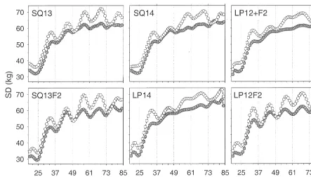
data. 2). Shifting knots by one month, however, made a quadratic approximation for intervals of this length 3.4. Alternative curves clearly inappropriate. At z56 and 9 RR coefficients, likelihoods for models SQ9.E1 and SQ9.E66 were While RR on orthogonal polynomials proved considerably lower than for SQ8.E1.
capable of modelling the cyclic, seasonal variation in Choice of knots was less critical when considering variance encountered in the data, high orders of quadratic approximation in 6 months segments. For polynomial fit were required. This resulted in a large PH, model SQ14.E1 gave a significantly better fit to number of parameters to be estimated and corre- the data than SQ13.E1, while for WOK SQ13.E1, spondingly large computational requirements. Other fitting 14 parameters less than SQ14.E1, produced a curves might be more suitable for this kind of higher log +. The latter indicates convergence
pattern, i.e. might provide similar results requiring problems for that analysis (SQ14.E1 in WOK). Both less RR to be fitted for each animal. models SQ13 and SQ14 yielded considerably higher
Segmented polynomials. The first alternative maximum log + values than LP14, at the same
considered were segmented polynomials. Such func- number (SQ14) or less (SQ13) parameters fitted, in tions have found occasional use in animal breeding both breeds (Table 2). As shown in Fig. 9, this was applications, e.g in modelling growth curves of goats clearly due to the greater scope of the SQ to follow (Gipson, 1997) or in describing lactation curves (El the cyclic changes of growth and its variation. Faro et al., 1998). More recently, there has been Differences in log + between SQ14 and LP14 were
2
interest in cubic spline functions to smooth lactation considerably less when fitting individual se (.E66)
2
curves (White et al., 1999); see also Verbyla et al. than when assuming homogeneous se, being 136.6 (1999) for a detailed exposition on the use of and 558.0, respectively, for PH and 126.6 and 443.9, smoothing splines for the analysis of longitudinal respectively, for WOK (Table 2). This suggested that data in a linear model framework. Allowing for part of the advantage of SQ over LP was due to different polynomials in individual segments, these being able to better account for differences in functions were expected to be more flexible in temporary environmental variation.
approximating the seasonally fluctuating growth Convergence of the SQ analyses was markedly curves in our data than polynomials fitted to the slower than that of corresponding LP analyses. whole range of ages. There has been concern about Presumably this was due to the fact that ordinary the numerical stability of covariance function esti- polynomials (5quadratics) were used which, by mates involving high orders of fit and thus high default, were highly correlated. Similarly, analyses powers of age (Kirkpatrick et al., 1994). Typically, fitting segmented cubic polynomials (SC9 and SC14) this created ‘wiggly’ surfaces when plotting esti- were unsuccessful, resulting in log + which were
mated covariances in the data, especially at the considerably lower than those of corresponding extremes of the ages considered. Fitting segments of analyses fitting quadratic functions (SQ8 and SQ13). low order polynomials was anticipated to have the This may well have been a convergence and parame-additional benefit of being less susceptible to such terisation problem. Perhaps an alternative representa-problems. tion would aid convergence. For instance, cubic Knots, i.e. joining points between segments were splines are seldom presented in the form of (5) but chosen after inspecting results from univariate analy- are often specified in a ‘value and second derivative’ ses and RR analyses involving Legendre polyno- at each knot form.
mials. Choosing segments of 12 months duration Fourier series approximation. The cyclic pattern
Fig. 9. Estimates of phenotypic standard deviations (in kg) for Polled Herefords (d) and Wokalups (s) from analyses fitting segmented
quadratic polynomials and Legendre polynomials superimposed by sinusoid and cosinoid curves, assuming homogeneous measurement error variances.
made an approximation by sinusoidal curves with a those for LP at very high orders of fit (k520, 22); periodicity of 12 months an obvious choice. Allow- see Figs. 5 and 8 for comparison. Correlations ing for covariances between all regression coeffi- between RR coefficients on LPs and RR on sine or cients, a model superimposing a Fourier series cosine curves were generally weak and on average approximation consisting of f curves onto Legendre close to zero. For analysis LP14F2.E1 in PH, for polynomials fitted to order k, LPkFf.Em, involved the instance, the 28 correlations ranged from 20.39 to same number of parameters as a model LP(k1f ).Em 0.38 with an average of 0.08. Assuming the two (at equal m). As shown in Table 2, a minimum order types of regression coefficients were uncorrelated of fit of k510 for LPs was required, sufficient to (models Pp1Ff ) resulted in dramatically increased describe the average trend in growth without distor- log + over values for the base polynomial function
tion, before models LPkFf.E1 fitted the data better (Pp) while adding only f( f11) / 2 covariances to be than their counterparts LP(k1f ).E1. Most of the estimated. For LP121F2.E1 and LP141F2.E1 in improvement in fit was achieved by fitting only one PH, for example, increases in log + over LP12.E1
sine and one cosine curve ( f52). While increasing f and LP14.E1 were as large as 1233.3 and 1270.4, to 4 (or 6) at constant LPk increased log + sig- respectively, for 3 additional parameters (Table 2).
nificantly in all cases examined, at equal number of However, the resulting estimates of (sP) exhibited parameters models LPkF4 generally had substantially a very different pattern to those obtained from lower log + than LP(k12)F2. corresponding analyses assuming covariances were
SQ), with only a small proportion of variance instance, used covariance functions to model chang-between animals contributed by the covariance func- ing variation in test day of dairy cows records across tion pertaining to the Ff part of the model. This the lactation and production level parsimoniously, suggested that a large proportion of the benefit with days in milk and herd level as independent achieved in adding an uncorrelated set of regression variables. While month did not quite represent a coefficients on sine and cosine functions, was totally continuous, infinite-dimensional scale, regres-through better modelling of the temporary environ- sions on month of recording were fitted for each mental variation. Alas, fitting cyclic error variances animal in an attempt to separate seasonal and age-for analysis LP141F2 in PH, increased log + by determined variation in weight. As shown in Table 2,
389.2 (LP141F2.E12C vs. LP141F2.E1; Table 2), this was done using Legendre polynomials and indicating that this was only a partial explanation and Fourier series approximations. In all instances, co-that a better fit could be achieved by modelling variances with RR coefficients on age were assumed heterogeneous error variances explicitly. to be zero.
Again, fitting any additional function increased log 3.5. Random regression on month of recording + significantly throughout. Effects of the additional
set of regression coefficients were most pronounced While most RR model analyses in the literature for models involving low orders of fit for RR on age consider a single continuous, independent variable (Table 2). This is illustrated in Fig. 10 for models only, the approach readily accommodates multiple LP121M Pp.E1] versus models LP20PM Pp.E1.] ‘meta-meters’. Veerkamp and Goddard (1998), for There was little difference in estimates of sP
tween orders of fit for LPs of months, k56 and coefficients was to a large part due to better
model-k510, respectively. As shown in Table 2, when ling of temporary environmental variation. fitting models LPk1M LP10.E1, the matrix of co-]
variances between RR coefficients for months con- 3.6. Analyses on the logarithmic scale sistently had a reduced rank of only 7, indicating that
a full order fit for months represented an over- Results from analyses of data transformed to parameterisation. logarithmic scale for selected models are given in Estimates of sP fitting Legendre polynomials for Table 3. On the whole, differences between analyses RR on months of recording (1M LPk) were lower] corresponded to those of the untransformed data. than those obtained fitting a Fourier series approxi- Existence of a scale effect on variances had been mation for months (1M Ff ), substantially so for] noticed above (Fig. 2). Estimates of sP for model
k512 and to a lesser extent for k520; see Fig. 10. LP20.E12C are contrasted in Fig. 11 to corre-Values for log + from analyses fitting a regression sponding values from univariate analyses. Again
on sine and cosine functions of age (1Ff ) and those there was close agreement between analyses for fitting a corresponding regression on month estimates of se, the logarithmic transformation hav-(1M Ff ) as a second, independent set of RR] ing levelled out univariate estimates, especially for coefficients were very similar (Table 2). Further- PH. Estimates of the between animal components more, resulting estimates of sP for equal f were showed less differences than for the untransformed virtually indistinguishable (not shown). This empha- data; see Fig. 8 for comparison.
sizes the close confounding between age and month While estimates of between animal standard devia-of recording in these data. The difference between tions still exhibited a cyclic pattern, this was less models 1M LPk and models] 1M Ff also supports] distinct and following a clear annual cycle than the hypothesis above that the improvement in log + observed previously. Peaks became particularly
and fit of the model due to these additional RR prominent for older ages. On the whole, there was a
slight downward trend in variance for later ages, stone et al. (2000) found that parametric curves fitted indicating that the upwards trend in estimates on the the data best, but produced negative estimates of untransformed scale was associated with the increase genetic correlations between early and late lactation in average weight. As the cyclic pattern on the while RR on orthogonal polynomials did not. The logarithmic scale shows, seasonal variation in vari- rationale for concentrating on variances (or standard ances clearly could only partially attributed to scale deviations) in this study was that it seemed futile to effects. Moreover, Fig. 11 suggests that the non-size examine covariances, unless variances had been related, seasonal differences became more important modelled correctly.
at later ages, presumably because variation in the RR models proved well capable of describing the ability of cows to cope with dearth increased with existing, complex pattern of variation. Not requiring age. any prior knowledge about the shape of curves to be modelled, RR on orthogonal polynomials of age performed admirably. While they required more
4. Discussion parameters to achieve the same degree of fit
(mea-sured by log + values) than other curves, they
Results showed a seasonal pattern in growth of appeared to be least susceptible to convergence animals, determined by high winter rain falls and problems, even for analyses involving well over 200 summer droughts and corresponding levels of pasture parameters to be estimated. Alternative curves in-availability. With almost complete confounding be- volving segmented polynomials or sine and cosine tween age at weighing and season, average growth functions required knots to be specified or the curves showed a corresponding, sinuous pattern (Fig. assumption that a sinusoidal curve of given period-1). Fixed effects fitted, i.e. year-week-paddock of icity (12 months) was appropriate. Analyses for recording and a fixed, cubic regression on age, models involving segmented polynomials were gen-accounted for differences in mean weights, but had erally slow to converge. In a few cases there were little effect on variances (Fig. 2). doubts whether convergence was real and had indeed Analyses identified a distinct cyclic pattern in achieved a global maximum. Future work should variances, both between animals and for temporary consider the use of orthogonal (rather than ordinary) environmental effects. As a transformation to loga- polynomials to model individual segments, and rithmic scale showed, this could only in part be investigate the joint estimation of knots.
attributed to scale effects. This implied that there Attempts to separate age-determined from season-was substantial variation between animals in their ally influenced variation between animals by fitting reaction to seasonal effects. Moreover, seasonal an additional RR on polynomials of month of fluctuations in variance independent of size appeared recording failed. Clearly, with the degree of con-to become more pronounced at later ages (Fig. 11). founding between age and season in the data, there Modelling this variation adequately presented a was insufficient information to do so. Nevertheless, seemingly unending task. With considerable numbers the second set of RR coefficients invariably resulted of records per animal, log + values increased in a better fit of the model considered, presumably to
significantly whenever any additional parameters some extent by accounting for differences in tempor-were added, even though differences in estimates of ary environmental variation.
variances appeared insubstantial in various instances. Measurement error variances were clearly not Clearly, variances alone do not represent the whole homogeneous. The cyclic pattern found indicated picture, estimates of covariance functions provided that this heterogeneity was primarily due to seasonal by RR model analyses give a description of co- effects. A model fitting 12 different, cyclically variances between all ages in the data. These need to repeating components thus appeared adequate. When be taken into account before deciding on the ‘best’ comparing models involving the same type of curve model. In comparing parametric curves and ortho- (e.g. orthogonal polynomials), however, estimates of gonal polynomials of days in milk in RR analyses of the between animal components were little affected
2
tock breeding. In: Proc. Sixth World Congr. Genet. Appl.
orders of fit could be compared assuming a single
Livest. Prod., Vol. 23, Armidale, Australia, pp. 32–39.
component, thus reducing computational
require-Jamrozik, J., Schaeffer, L.R., 1997. Estimates of genetic
parame-ments. ters for a test day model with random regressions for
pro-duction of first lactation Holsteins. J. Dairy Sci. 80, 762–770. Jamrozik, J., Schaeffer, L.R., Dekkers, J.C.M., 1997. Genetic evaluation of dairy cattle using test day yields and random
5. Conclusions
regression model. J. Dairy Sci. 80, 1217–1226.
¨ ¨ ¨
Kettunen, A., Mantysaari, E., Stranden, I., Poso, J., Lidauer, M.,
Random regression models have been advocated 1998. Estimation of genetic parameters for first lactation test for the analysis of longitudinal records on livestock. day milk production using random regression models. In: Proc. This study demonstrates that they are well suited to Sixth World Congr. Genet. Appl. Livest. Prod., Vol. 23,
Armidale, Australia, pp. 307–311.
the analysis of growth data, even if it is subject to
Kirkpatrick, M., Hill, W.G., Thompson, R., 1994. Estimating the
seasonal variation which cannot be separated.
Re-covariance structure of traits during growth and aging,
illus-gression on orthogonal polynomials do not require
trated with lactations in dairy cattle. Genet. Res. 64, 57–69.
prior assumptions about the shape of curves to be Kirkpatrick, M., Lofsvold, D., Bulmer, M., 1990. Analysis of the modelled and can be recommended as general pur- inheritance, selection and evolution of growth trajectories. pose functions, especially if higher orders of fit are Genetics 124, 979–993.
Koenen, E.P.C., Groen, A.F., Gengler, N., 1999. Phenotypic
feasible.
variation in live-weight and live-weight changes of lactating Holstein-Friesian cows. Anim. Sci. 68, 109–114.
Laird, N.M., Ware, J.H., 1982. Random-effects models for
longi-Acknowledgements tudinal data. Biometrics 38, 963–974.
Meyer, K., 1998a. ‘‘DXMRR’’-a program to estimate covariance functions for longitudinal data by restricted maximum
likeli-This work was funded under grant SBEF.014 of
hood. In: Proc. Sixth World Congr. Genet. Appl. Livest. Prod.,
Meat and Livestock Australia (MLA). I am indebted
Vol. 27, Armidale, Australia, pp. 465–466.
to the Western Australian Department of Agriculture Meyer, K., 1998b. Estimating covariance functions for longi-for their data. tudinal data using a random regression model. Genet. Select.
Evol. 30, 221–240.
Meyer, K., 1998c. Modeling ‘repeated’ records: Covariance functions and random regression models to analyse animal
References breeding data. In: Proc. Sixth World Congr. Genet. Appl.
Livest. Prod., Vol. 25, Armidale, Australia, pp. 517–520. Abramowitz, M., Stegun, I.A., 1965. Handbook of Mathematical Meyer, K., 1999. Estimates of genetic and phenotypic covariance
Functions, Dover, New York. functions for postweaning growth and mature weight of beef Anderson, S., Pedersen, B., 1996. Growth and food intake curves cows. J. Anim. Breed. Genet. 116, 181–205.
for group-housed gilts and castrated male pigs. Anim. Sci. 63, Meyer, K., Carrick, M.J., Donnelly, B.J.P., 1993. Genetic parame-457–464. ters for growth traits of Australian beef cattle from a multi-Brotherstone, S., White, I.M.S., Meyer, K., 2000. Genetic model- breed selection experiment. J. Anim. Sci. 71, 2614–2622.
ling of daily milk yield using orthogonal polynomials and Olori, V.E., Hill, W.G., Brotherstone, S., 1999. The structure of the parametric curves. Anim. Sci. (in press). residual error variance of test day milk yield in random El Faro, L., Galvao de Albuquerque, L., Fries, L.A., 1998. regression models. In: Proc. Computational Cattle Breeding
Adjusting lactation curves with segmented polynomials. In: Workshop 1999. Tuusula, Finland. ˜
Proc. Sixth World Congr. Genet. Appl. Livest. Prod., Vol. 23, Rekaya, R., Carabano, M.J., Toro, M.A., 1999. Use of test day Armidale, Australia, pp. 411–414. yields for the genetic evaluation of production traits in Hol-Fuller, W.A., 1969. Grafted polynomials as approximating func- stein-Friesian cattle. Livest. Prod. Sci. 34, 23–34.
tions. Austr. J. Agric. Econ. 13, 35–46. Schaeffer, L.R., Dekkers, J.C.M., 1994. Random regressions in Gallant, A.R., Fuller, W.A., 1973. Fitting segmented polynomial animal models for test-day production in dairy cattle. In: Proc. regression models whose join points have to be estimated. J. Fifth World Congr. Genet. Appl. Livest. Prod., Vol. 18, pp.
Amer. Stat. Ass. 68, 140–147. 443–446.
Stram, D.A., Lee, J.W., 1994. Variance component testing in the Veerkamp, R.F., Thompson, R., 1999. A covariance function for longitudinal model. Biometrics 50, 1171–1177. feed intake, live weight and milk yield estimated using a Tijani, A., Wiggans, G.R., Van Tassell, C.P., Philpot, J.C.M., random regression model. J. Dairy Sci. 82, 1265–1273.
Gengler, N., 1999. Use of (co)variance functions to describe Verbyla, A.R., Cullis, B.R., Kenward, M.G., Welham, S.J., 1999. (co)variances for test day yield. J. Dairy Sci. 82, On-line The analysis of designed experiments and longitudinal data by section, http: / / www.adsa.uiuc.edu / manuscripts / 8058. using smoothing splines (with discussion). Appl. Stat. 48, Van der Werf, J., Goddard, M., Meyer, K., 1998. The use of 269–311.
covariance functions and random regression for genetic evalua- White, I.M.S., Thompson, R., Brotherstone, S., 1999. Genetic and tion of milk production based on test day records. J. Dairy Sci. environmental smoothing of lactation curves with cubic
81, 3300–3308. splines. J. Dairy Sci. 82, 632–638.
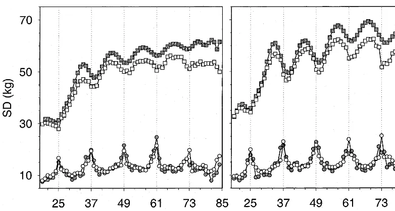
![Fig. 10. Estimates of phenotypic standard deviations (in kg) for Polled Herefords from analyses fitting random regressions on month ofrecording (m: Legendre polynomials with order of fit 6 (Model LPk1M LP6.E1), �: Legendre polynomials with order of fit 10 (ModelLPk]1M LP10.E1), d: Fourier series approximation with f 5 2 curves (Model LPk1F2.E1), and + : no regression for month (ModelLPk.E1))] in addition to regressions on Legendre polynomials of age, for order of fit of k 5 12 (left graph) and k 5 20 (right graph), assuminghomogeneous measurement error variances.](https://thumb-ap.123doks.com/thumbv2/123dok/1050918.933046/16.612.73.471.354.600/regressions-ofrecording-polynomials-polynomials-approximation-polynomials-assuminghomogeneous-measurement.webp)