Full Terms & Conditions of access and use can be found at
http://www.tandfonline.com/action/journalInformation?journalCode=ubes20
Download by: [Universitas Maritim Raja Ali Haji] Date: 11 January 2016, At: 22:07
Journal of Business & Economic Statistics
ISSN: 0735-0015 (Print) 1537-2707 (Online) Journal homepage: http://www.tandfonline.com/loi/ubes20
Should Macroeconomic Forecasters Use Daily
Financial Data and How?
Elena Andreou , Eric Ghysels & Andros Kourtellos
To cite this article: Elena Andreou , Eric Ghysels & Andros Kourtellos (2013) Should Macroeconomic Forecasters Use Daily Financial Data and How?, Journal of Business & Economic Statistics, 31:2, 240-251, DOI: 10.1080/07350015.2013.767199
To link to this article: http://dx.doi.org/10.1080/07350015.2013.767199
View supplementary material
Accepted author version posted online: 01 Feb 2013.
Submit your article to this journal
Article views: 898
View related articles
Should Macroeconomic Forecasters Use Daily
Financial Data and How?
Elena A
NDREOUDepartment of Economics, University of Cyprus, CY 1678 Nicosia, Cyprus ([email protected])
Eric G
HYSELSDepartment of Economics, University of North Carolina, Chapel Hill, NC 27599-3305, and Department of Finance, Kenan-Flagler Business School, Chapel Hill, NC 27599 ([email protected])
Andros K
OURTELLOSDepartment of Economics, University of Cyprus, CY 1678 Nicosia, Cyprus ([email protected])
We introduce easy-to-implement, regression-based methods for predicting quarterly real economic activity that use daily financial data and rely on forecast combinations of mixed data sampling (MIDAS) regressions. We also extract a novel small set of daily financial factors from a large panel of about 1000 daily financial assets. Our analysis is designed to elucidate the value of daily financial information and provide real-time forecast updates of the current (nowcasting) and future quarters of real GDP growth.
KEY WORDS: Daily financial factors; Financial markets and the macroeconomy; MIDAS regressions.
1. INTRODUCTION
Theory suggests that the forward-looking nature of finan-cial asset prices should contain information about the future state of the economy and therefore should be considered as extremely relevant for macroeconomic forecasting. Nowadays, a huge number of financial time series is available on a daily basis. Yet, to take advantage of the financial data-rich envi-ronment, one faces essentially two key challenges. The first challenge is how to handle the mixture of sampling frequen-cies, that is, matching daily (or an arbitrary higher frequency such as potentially intra-daily) financial data with quarterly (or monthly) macroeconomic indicators when one wants to predict short as well as relatively long horizons, like one year ahead. The second challenge is how to summarize the information or extract the common components from the vast cross-section of (daily) financial series that span the—in our analysis—five ma-jor classes of assets: commodities, corporate risk, equities, fixed income, and foreign exchange. In this article, we address both challenges.
To deal with data sampled at different frequencies, we use mixed data sampling (MIDAS) regressions. Recent surveys on MIDAS regressions and their use appear in Armesto, Engemann, and Owyang (2010); Andreou, Ghysels, and Kourtellos (2011); and Ghysels and Valkanov (2012). A number of recent articles have documented the advantages of using MIDAS regressions in terms of improving quarterly macro forecasts with monthly data, or improving quarterly and monthly macroeconomic pre-dictions with a small set (typically one or a few) of daily financial series. Notable examples include Clements and Galv˜ao (2008); Hamilton (2008); Schumacher and Breitung (2008); Ghysels and Wright (2009); Armesto et al. (2009); Clements and Galv˜ao (2009); Frale et al. (2011); Kuzin, Marcellino, and Schumacher (2011,2012); and Monteforte and Moretti (2012). These stud-ies, however, address neither the question of how to handle the information in large cross-sections of high-frequency financial
data, nor the potential usefulness of such series for real-time forecast updating.
To deal with the potentially large cross-section of daily series, we propose two approaches: (1) to reduce the dimensionality of the large panel, we extract a small set of daily financial factors from a large cross-section of around 1000 financial time series and a substantially smaller cross-section of financial predictors proposed in the literature, which cover the five aforementioned asset classes, and (2) we apply forecast combination methods to these daily financial factors as well as to the smaller cross-section of individual daily financial predictors to provide robust and accurate forecasts for economic activity.
The article is organized as follows. In Section2, we describe the MIDAS regression models. Section3discusses the quarterly and daily data. In Section4, we present the factor analysis and forecast combination methods. In Section5, we present the em-pirical results, which include comparisons of MIDAS regression models with daily financial data and traditional models using ag-gregated data as well as models with leads in macroeconomic and financial data. Section6concludes.
2. MIDAS REGRESSION MODELS
Suppose we wish to forecast a variable observed at some low frequency, say for one quarter ahead, denoted by YtQ+1, such as, for instance, real GDP growth, and we have at our disposal financial series that are considered as useful predictors. Denote by XtQ a quarterly aggregate of a financial predictor series (the aggregation scheme being used is, say, averaging of the data available daily). One conventional approach is to use an
© 2013American Statistical Association Journal of Business & Economic Statistics April 2013, Vol. 31, No. 2 DOI:10.1080/07350015.2013.767199
240
Augmented Distributed Lag, ADL(pQY, qXQ), regression model: gression is fairly parsimonious as it only requirespYQ+qXQ+1 regression parameters to be estimated. Assume now that we would like to use instead the daily observations of the financial predictor seriesXt.Denote byXDm−j,tthejth day counting back-ward in quartert.Hence, the last day of quartertcorresponds withj =0 and is therefore XDm,t, where mdenotes the daily lags or the number of trading days per quarter—assumed to be constant for the sake of simplicity.
Generalizing the above argument toh-steps ahead forecasts, we get the ADL-MIDAS(pYQ, qD
X) regression model given by
YtQ,h+h =µh+
where the weighting scheme involves a low-dimensional vector of unknown hyperparametersθto avoid the parameter prolifer-ation issue implied by having to estimate a coefficient for each high-frequency lag. This model can be used to obtain direct (as opposed to iterated) forecasts for multiperiods ahead. Note that to simplify notation and exposition, we take quarterly blocks of daily data as lag. In effect, the ADL-MIDAS regression model generalizes the standard ADL forecasting approach [e.g., Stock and Watson (2003)] to tackle mixed-frequency data.
There are several possible parameterizations of the MIDAS polynomial weights including, for example, the U-MIDAS (unrestricted MIDAS polynomial), normalized Beta proba-bility density function, normalized exponential Almon lag polynomial, and polynomial specification with step functions. Ghysels, Sinko, and Valkanov (2006) provided a discussion on the alternative weighting schemes. Following Ghysels, Sinko, and Valkanov (2006), we use an exponential Almon lag polynomial that features positive weights, which sum to one. The latter restriction allows the identification of the parameter
βh. In particular, we use wθjh =mexp(θhj2)
j=1exp(θ2hj2) which further
restricts the weighting scheme to linear or downward sloping shapes so that we only have to estimate one hyperparameter,
θh, which is especially useful in our context given the relatively small sample size of our data. We found that this particular parameterization yields a parsimonious, yet flexible scheme of data-driven weights. In unreported exercises, we have also experimented with a two-parameter exponential Almon lag polynomial without finding any forecasting improvements. The MIDAS modeling approach allows us to obtain a linear projection of high-frequency dataXtDontoYtQwith a small set of parameters. The parameters, (µh, ρh
of the MIDAS regression model in Equation (2.2) are estimated by nonlinear least squares [when m is small—for example, in the quarterly/monthly setting—one can use a U-MIDAS specification and use ordinary least squares (OLS), suggested by Foroni, Marcellino, and Schumacher (2011)].
2.1 Temporal Aggregation Issues
It is worth pointing out that there is a more subtle relationship between the ADL regression appearing in Equation (2.1) and the ADL-MIDAS regression in Equation (2.2). Note that the ADL regression involves temporally aggregated series, based, for example, on equal weights of daily data, that is, XQt = (XD1,t+XD2,t+ · · · +XDm,t)/m.
If we take the case ofmdays of past daily data in an ADL regression, then implicitly through aggregation we have picked the weighting scheme β1/mfor the daily data X.,tD. We will sometimes refer to this scheme as a flat aggregation scheme. While these weights have been used in the traditional temporal aggregation literature, they may not be optimal for time series data, which most often exhibit a downward sloping memory decay structure, or for the purpose of forecasting as more recent data may be more informative and thereby get more weight. In general though, the ADL-MIDAS regression lets the data decide the shape of the weights.
We can relate MIDAS models to the temporal aggregation literature and ADL models by considering the following filtered parameter-drivenquarterlyvariable: where M in the model’s acronym refers to the fact that the model involves a multiplicative weighting scheme, namely,
YtQ,h+h =µh+
At this point, several issues emerge. Some issues are theoret-ical in nature. For example, to what extent is this tightly param-eterized formulation in Equation (2.2) able to approximate the unconstrained (albeit practically infeasible) projection? There is also the question of how the regression in Equation (2.2) relates to the more traditional approach involving the Kalman filter. We do not deal directly with these types of questions here, as they have been addressed notably in Bai, Ghysels, and Wright (2010). However, some short answers to these questions are as follows.
First, it turns out that MIDAS regression models can be viewed as a reduced form representation of the linear projection that emerges from a state-space model approach [see Bai, Ghysels, and Wright (2010) for further discussion]. Second, the Kalman filter, while clearly optimal as far as linear projections in a Gaussian setting go, has some disadvantages, namely, (1) it is more prone to specification errors as a full system of equations and latent factors are required and (2) it requires a lot more pa-rameters to achieve the same goal. Therefore, the Kalman filter approach is often feasible when dealing with a small system of mixed frequencies [such as, for instance, Aruoba, Diebold, and Scotti (2009), which involves only six series]. Instead, our analysis deals with a larger number of daily variables (ranging from 64 to 991), and therefore the approach we propose is regression-based and reduced form—notably not requiring to model the dynamics of each and every daily predictor series
and estimate a large number of parameters. Consequently, our approach deals with a parsimonious predictive equation, which in most cases leads to improved forecasting ability.
2.2 Nowcasting and Leads
Nunes (2005) and Giannone, Reichlin, and Small (2008), among others, have formalized the process of updating forecasts as new releases of data become available, using the terminology of nowcasting for such updating. In particular, using a dynamic factor state-space model and the Kalman filter, one models the joint dynamics of real GDP and the monthly data releases and proposes solutions for estimation when data have missing ob-servations at the end of the sample due to nonsynchronized publication lags (the so-called jagged/ragged edge problem).
In this article, we propose an alternative reduced form strategy based on MIDAS regressions with leads, introduced by Clements and Galv˜ao (2008) and Kuzin, Marcellino, and Schumacher (2012) in the context of monthly–quarterly data mixtures, to incorporate real-time information of daily finan-cial variables. There are two important differences between nowcasting (using the Kalman filter) and MIDAS with leads. Before we elaborate on these two differences, we explain first what is meant by MIDAS with leads.
The notion of leads pertains to the fact that we use information between t and t+1. Suppose we are 2 months into quarter
t+1,hence the end of February, May, August, or November, and our objective is to forecast quarterly economic activity. This implies we often have the equivalent of at least 44 trading days (2 months) of daily financial data. Denote by XDm−i,t+1 the ith day counting backward in quartert+1 and consider
JXD daily leads for the daily predictor in terms of multiples of months,JXD =1 and 2. For example, in the case ofJXD =2,
XD2m/3,t+1corresponds to 44 leads, whileX D
1,t+1corresponds to 1 lead for the daily predictor. Then we can specify the ADL-MIDAS(pQY, qD
It should be noted that there are various ways to hyperpara-meterize the lead and lag MIDAS polynomials. In addition, the common slope,βh, restriction may also be relaxed in Equation (2.5). This results in quite a few variations in the specification of the MIDAS regression model, in particular when combined with the various polynomials. For a complete list of MIDAS regression models, we refer the reader to Andreou, Ghysels, and Kourtellos (2012)—henceforth, we will refer to this as the Internet Appendix.
The first difference between nowcasting and MIDAS with leads can be explained as follows. Typically nowcasting refers to within-period updates of forecasts. An example would be the frequent updates ofcurrentquarter real GDP forecasts. MIDAS with leads can be viewed as current quarter updates not only of current quarter real GDP forecasts, but also of any future
horizon real GDP forecast (i.e., over several future quarters). While both state-space and MIDAS models can produce multi-ple horizon forecasts, a subtle difference is that MIDAS mod-els can produce direct (as opposed to iterated) h-step ahead forecasts. Arguably iteration-based forecasts can suffer from misspecification, which can be compounded across multiple horizons that may produce inferior forecasts; see, for example, Marcellino, Stock, and Watson (2006).
The second difference between typical applications of now-casting and MIDAS with leads pertains to the jagged/ragged edge nature of macroeconomic data. Nowcasting addresses the real-time nature of macroeconomic releases directly—the nature being jagged/ragged edged as it is referred to due to the unevenly timed releases. Hence, the release calendar of macroeconomic news plays an explicit role in the specification of the state-space measurement equations. Potentially, MIDAS regressions with leads in macroeconomic data can also address the ragged char-acter of such series. However, given that the focus of this article is the high-frequency daily financial data, we do not constantly update the low-frequency macro series. Stated differently, our approach puts the trust into the financial data in absorbing and impounding the latest news into asset prices. There is obviously a large literature in finance on how announcements affect fi-nancial series. The daily flow of information is absorbed by the financial data being used in MIDAS regressions with leads— which greatly simplifies the analysis. The Kalman filter in the context of nowcasting has the advantage that one can look at how announcement “shocks” affect forecasts. While it may not be directly apparent, MIDAS regressions with leads can provide similar tools. It suffices to run MIDAS regressions with leads using prior and postannouncement financial data and to analyze the changes in the resulting forecasts [see, e.g., Ghysels and Wright (2009) for further discussion].
It should also be noted that traditional nowcasting not only deals with the very detailed calendar of macroeconomic re-leases, it also keeps track of data revisions. The MIDAS with leads in financial data has the advantage of using financial data that are observed without measurement error and are not subject to revisions as opposed to most macroeconomic indicators. In some sense, we let the financial markets absorb the news and use the market discovery process to our advantage when ap-plying MIDAS regressions based on daily financial series. We should also note that MIDAS regression models with leads in financial data can easily be extended to incorporate leads and lags in macroeconomic data using a different MIDAS polyno-mial. In this article, we attempt a limited number of exercises that aim at comparing the MIDAS regression models with leads in financial data against alternative specifications that allow for leads in macroeconomic data or both, discussed in detail below.
3. DATA
We focus on forecasting the U.S. quarterly real GDP growth rate and study two sample periods. A longer sample period from January 1, 1986, to December 31, 2008 (of 92 quarters or 4584 trading days), and a shorter subperiod from January 1, 1999, to December 31, 2008 (of 40 quarters or 1777 trading days). These samples will henceforth throughout the article be called long sample and short sample, respectively. Most of our analysis
focuses on the long sample, but there are at least two reasons why we also choose to analyze the shorter sample. First, this period provides a set of daily financial predictors that is new rel-ative to most of the existing literature on forecasting, including new series such as corporate risk spreads (e.g., the A2P2F2 mi-nus AA nonfinancial commercial paper spreads), term structure variables (e.g., inflation compensation series or break-even in-flation rates), and equity measures [such as the implied volatility of S&P500 index option (VIX), the Nasdaq 100 stock market returns index]. These predictors are not only related to eco-nomic models, which explain the forward looking behavior of financial variables for the macro state of the economy, but have also been recently informally monitored by policy makers and practitioners even on a daily basis to forecast inflation and eco-nomic activity. Examples include the break-even inflation rates discussed during the Federal Open Market Committee meetings and the VIX index often coined as the stock market fear-index. Second, we note that this recent period belongs to the post-1985 Great Moderation era, which is marked as a structural break in many U.S. macroeconomic variables and has been documented that it is more difficult to predict such key macroe-conomic variables (D’Agostino, Surico, and Giannone 2007) vis-`a-vis simple univariate models such as the random walk (RW) for economic growth compared with the pre-1985 period. Therefore, we take the challenge of predicting economic growth in a period that many models and methods did not provide sub-stantial forecasting gains over simple models.
We use three databases at different sampling frequencies: daily, monthly, and quarterly. The daily database includes a large cross-section of 991 daily series for five classes of finan-cial assets. We use this large dataset to extract a small set of daily financial factors. The five classes of daily financial as-sets are (i) the commodities class, which includes 241 variables such as U.S. individual commodity prices, commodity indices, and futures; (ii) the corporate risk category includes 210 vari-ables such as yields for corporate bonds of various maturities, LIBOR (London Interbank Offered Rate), certificate of deposits, Eurodollars, commercial paper, default spreads using matched maturities, quality spreads, and other short-term spreads such as TED; (iii) the equities class comprises 219 variables of the ma-jor international stock market returns indices and Fama-French factors and portfolio returns as well as U.S. stock market vol-ume of indices and option volatilities of market indices; (iv) the foreign exchange rates class includes 70 variables such as major international currency rates and effective exchange rate indices; and (v) the government securities class includes 248 variables of government treasury bonds rates and yields, term spreads, treasury inflation-protected securities yields, and break-even inflation.
Unfortunately, most of these 991 daily financial assets are only available for the short sample. For the long sample, we only observe 64 daily financial assets including 27 commodity variables, 9 corporate risk series, 11 equity series, 6 foreign exchange series, and 11 government securities. Most of these daily predictors have been proposed in the literature as good predictors of economic growth. For the short sample, we inves-tigate two more targeted subsets from the large cross-section, a set of 92 daily assets, and a subset of 64 daily assets that matches the predictors of the long sample. The motivation for
adding the additional 18 predictors in the sample of 92 daily predictors for the short period is based on recent studies, for example, Edelstein (2007) used a set of commodities to predict U.S. inflation, G¨urkaynak, Sack, and Wright (2010) proposed new data on break-even inflation, and Buchmann (2011) em-ployed a set of Euro area Merill Lynch corporate bond spreads vis-`a-vis the long-run government bond spreads.
The daily database also includes the ADS (Aruoba-Diebold-Scott) Business Conditions Index proposed by Aruoba, Diebold, and Scotti (2009), which is a daily factor. This factor is based on six U.S. macroeconomic nonfinancial variables of mixed frequency (weekly initial jobless claims, monthly payroll em-ployment, industrial production, personal income less transfer payments, manufacturing and trade sales, and quarterly real GDP).
The monthly database includes three macroeconomic series, the Chicago Fed National Activity Index (CFNAI), the Institute for Supply Management Manufacturing: New Orders Index (NAPMNOI), and the Total Nonfarm Payroll Employment (EMPLOY). The choice of the CFNAI is based on the fact that it is a coincident indicator of the overall economic activity and it is computed as a weighted average of 85 monthly indicators of national economic activity drawn from four broad categories of data: (i) production and income; (ii) employment, unemployment, and hours; (iii) personal consumption and housing; and (iv) sales, orders, and inventories. The CFNAI is released toward the end of each calendar month with approximately 1 month delay. NAPMNOI and EMPLOY are more timely. NAPMNOI is released on the first business day of each month, and the Bureau of Labor Statistics typically announces EMPLOY on the first Friday of the month.
Finally, the quarterly database is an update of the database of Stock and Watson (2008b) with the difference that it excludes (fi-nancial) variables observed at the daily frequency, which were already included in the database of daily financial assets. In particular, it covers 69 variables including real output and in-come, capacity utilization, employment and hours, price indices, money, etc.
The data sources are Haver Analytics, which is a data ware-house that collects the data series from their original sources [such as the Federal Reserve Board (FRB), Chicago Board of Trade (CBOT), and others], the Global Financial Database (GFD), Chicago Fed, Philadelphia Fed, and FRB, unless other-wise stated. All the series were transformed to eliminate trends so as to ensure stationarity. Detailed description of the three databases including information about the transformations can be found in the Internet Appendix. For all series with revisions, the May 2009 vintage is used.
4. IMPLEMENTATION ISSUES
In this section, we develop two complementary approaches to address the use of a large cross-section of high-frequency financial data. The first approach extracts factors from cross-sections observed at different frequencies described in Section3. The second approach involves forecast combinations of MIDAS regressions with a single daily financial asset or factor. We use the two approaches as complementary rather than competing in the sense that we employ forecast combinations of both daily
financial assets and daily financial factors. Forecast combi-nations deal explicitly with the problem of model uncertainty by obtaining evidentiary support across all forecasting models rather than focusing on a single model.
4.1 Daily and Quarterly Factors
There is a large recent literature on dynamic factor model (DFM) techniques that are tailored to exploit a large cross-sectional dimension; see, for instance, Bai and Ng (2002,2003); Forni et al. (2000,2005); and Stock and Watson (1989,2003), among many others. The idea is that a handful of unobserved common factors are sufficient to capture the covariation among economic time series. Typically, the literature estimates these factors at low frequency (e.g., quarterly) using a large cross-section of time series. Then these estimated factors augment the standard autoregressive (AR) and ADL models to obtain the factor AR (FAR) and factor ADL (FADL) models, respectively. In fact, Stock and Watson (2002b,2006) found that such models can improve forecasts of real economic activity and other key macroeconomic indicators based on low-dimensional forecast-ing regressions.
Following this literature, we obtain quarterly macroeconomic factors and daily financial factors for both the long and the short sample using the principal component approach. Our analysis is based on a DFM with time-varying factor loadings of Stock and Watson (2002a). The choice of a DFM is based on two main reasons. First, the errors of the DFM could be conditionally heteroscedastic and serially and cross-correlated [see Stock and Watson (2002a) for the full set of assumptions]. These assump-tions are relevant given that most daily financial time series exhibit GARCH (generalized autoregressive conditional het-eroscedasticity) type dynamics. Second, the DFM can allow the factor loadings to change over time, which may address potential instabilities during our sample period [see theorem 3, p. 1170, in Stock and Watson (2002a)]. Hence, the extracted common factors can be robust to instabilities in individual time series, if such instability is small and sufficiently dissimilar among in-dividual variables, so that it averages out in the estimation of common factors.
In particular, the quarterly macroeconomic factors are based on the quarterly database of 69 real macroeconomic series, which as noted in Section 3, excludes the financial variables from the database of Stock and Watson (2008b). Hence, we call these quarterly factors as the Stock & Watson (S&W) (real) macroeconomic factors. Alternatively, we use the quarterly aver-age of the monthly CFNAI factor, which is based on an extension of the methodology used to construct the original S&W factors. Given that we will be using the monthly CFNAI factor in models with leads in macroeconomic data, we find it useful to consider this alternative quarterly factor, too. The daily financial factors are extracted from (i) the 64 daily financial assets of the long sample, (ii) the entire large cross-section of 991 daily financial series of the short sample, and (iii) each of the 5 homogeneous classes of financial assets of the short sample.
There are alternative approaches to choosing the number of factors. One approach is to use the information criteria (ICp) proposed by Bai and Ng (2002). For the quarterly macroe-conomic factors, ICp criteria yield two factors for the period
1999:Q1–2008:Q8, denoted by F1Q and F2Q. These first two quarterly factors explain 36% and 12%, respectively, of the total variation of the panel of quarterly variables. The first quarterly factor correlates highly with Industrial Production and Purchas-ing Manager’s index, whereas the second quarterly factor corre-lates highly with Employment and the NAPM inventories index. These results are consistent with Stock and Watson (2008a) who used a longer time-series sample as well as Ludvigson and Ng (2007,2009) who used a different panel of U.S. data. Inter-estingly, although our quarterly database excludes 20 financial variables from the original Stock and Watson database that are available at daily frequency, our first two factors correlate al-most perfectly with those of Stock and Watson (with correlation coefficients equal to 0.99 and 0.98 for factors 1 and 2, respec-tively). Hence, the excluded 20 aggregated financial series do not seem to play an important role for extracting the first two factors for the period 1999:Q1–2008:Q4.
For the daily financial factors, we find that all three ICp crite-ria always suggest the maximum number of factors. Therefore, to choose the number of daily factors, we assess the marginal contribution of thekth principal component in explaining the total variation. We opt to use all five daily factors since we have found that overall this number explains a sufficiently large per-centage of the cross-sectional variation. All the details on the standardized eigenvalues and loadings are found in the Internet Appendix.
Once we obtained the quarterly macroeconomic factors and daily financial factors, we investigate their predictive roles using MIDAS regression models. In particular, the MIDAS regression models in Equations (2.2), (2.4), and (2.5) are augmented with the vector of quarterly factors,FQ, which includes either the two S&W factors or the CFNAI factor. For example, Equation (2.2) generalizes to FADL-MIDAS(pQY, qFQ, qXD) model
YtQ,h+h =µ h
+
pYQ−1
k=0
ρkhYtQ−k+ qFQ−1
k=0
αkh′FtQ−k
+βh qD
X−1
j=0 m−1
i=0
wiθ+hj∗mX D
m−i,t−j+u h
t+h. (4.1)
It is worth noting that the above equation simplifies to the traditional FADL when the MIDAS features are turned off— that is, say, a flat aggregation scheme is used.
Finally, we investigate the predictive role of the daily financial factors,FD, using ADL-MIDAS and FADL-MIDAS regression models. For reasons of parsimony, we only consider forecasting models that include the daily financial factors one at a time. Essentially, in these models, the daily financial factor plays the role of the daily predictor, XD. This kind of analysis shifts the focus from unconditional statements about the number of factors to conditional statements about the predictive ability of daily factors.
4.2 Forecast Combinations
There is a large and growing literature that suggests that fore-cast combinations can provide more accurate forefore-casts by using evidence from all the models considered rather than relying on a
specific model. Timmermann (2006) provided an excellent sur-vey of forecast combination methods. One justification for using forecast combinations methods is the fact that in many cases, we view models as approximations because of the model uncer-tainty that forecasters face due to the different set of predictors, the various lag structures, and generally the different modeling approaches. Furthermore, forecast combinations can deal with model instability and structural breaks under certain conditions and simple strategies such as equally weighting schemes (Mean) can produce more stable forecasts than individual forecasts [e.g., Hendry and Clements (2004); Stock and Watson (2004)]. In contrast, Aiolfi and Timmermann (2006) showed that combination strategies based on some presorting into groups can lead to better overall forecasting performance than simpler ones in an environment with model instability. Although there is a consensus that forecast combinations improve forecast accu-racy, there is no consensus concerning how to form the forecast weights.
The forecast combination ofYtQ,h+h made at timetis a (time-varying) weighted average ofMindividualh-step ahead out-of-sample forecasts, (Y1Q,h,t+h, . . . ,Y
Q,h
M,t+h), given as
YcQ,h
M,t+h=
M
i=1
ωhi,tYi,tQ,h+h, (4.2)
where (ωhi,t, . . . , ωhM,t) is the vector of combination weights formed at time t; cM emphasizes the fact that the combined forecast depends on the model space or set of individual fore-casts.
While there are several methods to estimate the combination weights, in this article we focus on the squared discounted mean squared forecast error (MSFE) combinations method, which yields the highest forecast gains relative to other methods in our samples; see also Stock and Watson (2004,2008b). This method accounts for the historical performance of each individual by computing the combination forecast weights that are inversely proportional to the square of the discounted MSFE with a high discount factor attaching greater weight to the recent forecast accuracy of the individual models. More generally, the weights are given as follows:
ωi,th = λ −1 i,t
κ
n
j=1(λ −1 j,t)κ
, λi,t=
t−h
τ=T0
δt−h−τ YQ,h τ+h−Y
Q,h i,τ+h
2
,
(4.3)
whereδ=0.9 andκ=2. Following Stock and Watson (2008b), we also report in the Internet Appendix a number of alterna-tive forecast combination methods including an alternaalterna-tive dis-counted MSFE (withδ =0.9 andκ =1), the Recently Best, the Mean, the Median, and the Mallows Model Averaging (MMA) method. T0 is the point at which the first individual pseudo out-of-sample forecast is computed. For the long sample,T0= 2001:Q1, while for the short sample,T0=2006:Q1.
Operationally, we compute forecasts for various families of models with single predictors using daily, monthly, and quarterly data to evaluate the predictive role of daily financial assets and factors. More precisely, we proceed in three steps. First, for a given family of models and a given daily financial asset or factor, we compute forecasts using several models with
alternative lag structures based on both a fixed lag length scheme and AIC-based criterion. Second, for each asset, we select the best model specification in terms of its out-of sample perfor-mance in pseudo real time. And third, given a family of models, we deal with uncertainty with respect to the predictors by com-bining forecasts from models with alternative assets or financial factors. One implication of this strategy is that our tests for com-paring among families of the combined models can be viewed as nonnested. For example, when comparing forecast combi-nations of individual FADL-MIDAS against FADL models, the comparison is nonnested because the two families of models can involve individual models with different lag structures.
5. EMPIRICAL RESULTS
Using a recursive estimation method, we provide pseudo out-of-sample forecasts [see also, for instance, Stock and Watson (2002b,2003)] to evaluate the predictive ability of our mod-els. The total sample size,T +h, is split into the period used to estimate the models, and the period used for evaluating the forecasts. The initial estimation periods for the long and short samples are 1986:Q1 to 2000:Q4 and 1999:Q1 to 2005:Q4, while the forecasting periods are 2001:Q1+h to 2008:Q4−h
and 2006:Q1+h to 2008:Q4−h, respectively. Although both samples are relatively small for nonlinear least squares esti-mation, it is comforting to note that Bai, Ghysels, and Wright (2010) provided some Monte Carlo simulation evidence that the predictive performance of MIDAS regression models may not be affected. In any event, we always compare the predictive ability of MIDAS regression models with the corresponding tra-ditional models that simply take an equally weighted average of daily indicators. We assess the forecast accuracy of each model using the root mean squared forecast error (RMSFE).
5.1 MIDAS Regression Models With Daily Financial Data
We begin our analysis by investigating whether MIDAS re-gression models with daily financial data are useful in fore-casting quarterly economic activity beyond macroeconomic data.Table 1presents RMSFEs for one- and four-quarter-ahead (h=1,4) forecasts using two samples, the long sample and the short sample. The analysis for the short sample, however, is restricted toh=1 due to the small number of observations. With the exception of the RMSFE of the RW, which is given in absolute values, all RMSFEs are expressed in ratios over the RW so that a ratio less than one is interpreted as an improvement of the underlying forecast upon the RW.
In particular, we investigate four families of models: (i) uni-variate models, (ii) models with macro factors, (iii) models with financial data, and (iv) models with macroeconomic and financial data. The last two families of models report forecast combination results for models with financial predictors or factors. For the long sample, we report forecast combination results on 64 daily financial assets (64 DA) and 5 daily financial factors (5 DF) extracted from these 64 daily predictors. For the short sample, we show forecast combinations of 92 daily financial assets (92 DA) as well as a subset of 64 daily predictors that matches the daily predictors of the long sample. It also
Table 1. RMSFE comparisons for models with no leads
Long sample Short sample
Forecast horizon h=1 h=4 h=1 h=4 h=1 h=1 h=1 h=1
Univariate models
RW 2.56 1.18 – – 3.35 – – –
AR 0.96 1.01 – – 1.00 – – –
Models with macro data
FAR (S&W) 0.84 0.96 – – 0.73 – – –
FAR (CFNAI) 0.83 0.98 – – 0.80 – – –
64 DA 5 DF 92 DA 64 DA 5 DF 25 DF
Models with financial data
ADL 0.88 0.92 0.88 0.90 0.90 0.92 0.79 0.80
ADL-MIDAS(JD
X =0) 0.80 0.89 0.87 0.86 0.79 0.81 0.66 0.79
Models with macro and financial data
FADL (S&W) 0.88 0.83 0.77 0.86 0.69 0.67 0.62 0.58
FADL (CFNAI) 0.77 0.88 0.80 0.89 0.68 0.67 0.61 0.65
FADL-MIDAS(JD
X =0) (S&W) 0.81 0.80 0.78 0.81 0.65 0.64 0.61 0.54
FADL-MIDAS(JD
X =0) (CFNAI) 0.72 0.86 0.79 0.85 0.65 0.64 0.59 0.64
NOTE: This table presents RMSFEs of forecast combinations for real GDP growth relative to the RMSFE of the RW for one- and four-step ahead forecasts for the long sample and one-step ahead forecasts for the short sample. It includes results on the benchmark models of the RW (in absolute values) and the AR as well as the FAR. The column headings DA and DF denote forecast combinations results on models with daily financial assets and daily financial factors, respectively. For the long sample, it includes forecast combination results on 64 DA and 5 DF extracted from those 64 daily predictors. For the short sample, it includes forecast combinations of 92 DA as well as a subset of 64 DA that matches the 64 DA of the long sample. It also includes forecast combination results on the 5 DF extracted from all 991 variables and the 25 DF obtained from the five homogeneous classes of assets (5 from each classes). The prefix “F” refers to models that include the quarterly CFNAI factor or the two S&W factors. The estimation periods for the long and short samples are 1986:Q1 to 2000:Q4 and 1999:Q1 to 2005:Q4, while the forecasting periods 2001:Q1+hto 2008:Q4−hand 2006:Q1+hto 2008:Q4−h, respectively. The entries less than 1 imply improvements over the RW benchmark.
includes forecast combination results on the 5 daily financial factors extracted from all 991 variables and the 25 daily financial factors (25 DF) obtained from the five homogeneous classes of assets (5 from each classes).
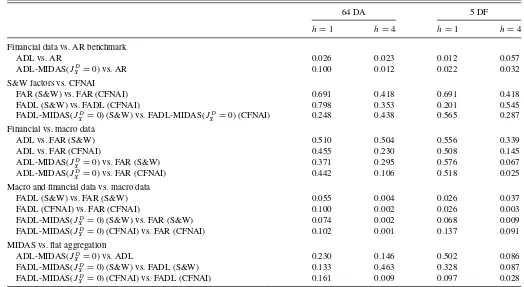
Table 2showsp-values for the null hypothesis of equal pre-dictive ability using the test of Diebold and Mariano (1995) and West (1996). These tests focus on the long sample and com-pare the predictive ability between selected families of models.
Table 2. Testing for equal predictive ability for models with no leads
64 DA 5 DF
h=1 h=4 h=1 h=4
Financial data vs. AR benchmark
ADL vs. AR 0.026 0.023 0.012 0.057
ADL-MIDAS(JD
X =0) vs. AR 0.100 0.012 0.022 0.032
S&W factors vs. CFNAI
FAR (S&W) vs. FAR (CFNAI) 0.691 0.418 0.691 0.418
FADL (S&W) vs. FADL (CFNAI) 0.798 0.353 0.201 0.545
FADL-MIDAS(JD
X =0) (S&W) vs. FADL-MIDAS(JXD=0) (CFNAI) 0.248 0.438 0.565 0.287
Financial vs. macro data
ADL vs. FAR (S&W) 0.510 0.504 0.556 0.339
ADL vs. FAR (CFNAI) 0.455 0.230 0.508 0.145
ADL-MIDAS(JD
X =0) vs. FAR (S&W) 0.371 0.295 0.576 0.067
ADL-MIDAS(JD
X =0) vs. FAR (CFNAI) 0.442 0.106 0.518 0.025
Macro and financial data vs. macro data
FADL (S&W) vs. FAR (S&W) 0.055 0.004 0.026 0.037
FADL (CFNAI) vs. FAR (CFNAI) 0.100 0.002 0.026 0.003
FADL-MIDAS(JD
X =0) (S&W) vs. FAR (S&W) 0.074 0.002 0.068 0.009
FADL-MIDAS(JD
X =0) (CFNAI) vs. FAR (CFNAI) 0.102 0.001 0.137 0.091
MIDAS vs. flat aggregation ADL-MIDAS(JD
X =0) vs. ADL 0.230 0.146 0.502 0.086
FADL-MIDAS(JD
X =0) (S&W) vs. FADL (S&W) 0.133 0.463 0.328 0.087
FADL-MIDAS(JD
X =0) (CFNAI) vs. FADL (CFNAI) 0.161 0.009 0.097 0.028
NOTE: This table reportsp-values of the two-sided hypotheses that compare the predictive ability between selected families of models reported inTable 1for the long sample. All comparisons are based on the Diebold–Mariano test.
The standard error is based on the sample variance for all fore-cast horizons, despite the fact that multistep forefore-cast errors are known to be serially correlated. The reason for doing so is the concern that heteroscedasticity and autocorrelation consistent (HAC) variance estimators that account for the serial correla-tion of the forecast errors can be generally imprecise for such small samples. Nevertheless, for robustness purposes, we also report in the Internet Appendix the corresponding tests using the adjusted variance developed by Harvey, Leybourne, and Newbold (1997), which is one of the estimators that performs relatively well in the small-sample Monte Carlo analysis of Clark and McCracken (2012). In general, results are qualita-tively similar.
A close examination of these tables reveals the following five results. First, we find that models that condition on financial assets alone improve the forecasting ability of the univariate AR. For example, in the case of the long sample, for the 64 DA, andh=1, the ADL and ADL-MIDAS improve upon the
AR by 8% and 17%, respectively. We find similar gains for the longer horizon, h=4, and for models with 5 DF. In the
case of the short sample and especially for the 5 DF, the gains are even stronger.Table 2shows the gains for the long sample are statistical significant at least at 5%.
Second, in general, we find that quarterly (real) macroeco-nomic factors play a major role in forecasting quarterly real GDP growth for both MIDAS and traditional models. To see this, we make two observations. For the long sample, we ob-serve that models with macro factors are strong competitors of models with financial predictors or factors especially forh=1. Although the ADL and ADL-MIDAS appear to perform bet-ter than the FAR models for h=4, we can only reject the null hypothesis of equal predictive ability between the FAR and the ADL-MIDAS using 5 DF. Additionally, all the FADL and FADL-MIDAS models provide forecasting gains over the corresponding ADL and ADL-MIDAS models for both sam-ples and horizons as well as for all the forecast combination cases. This finding is true irrespective of whether we use the single quarterly CFNAI factor or the two S&W factors, and it is also consistent with Stock and Watson (2002b), albeit using a different sample period, namely, 1959–1998. In fact, a test of equal predictive ability between models with S&W factors and models with CFNAI suggests that we can use these factors alternatively.
Third, the FADL and FADL-MIDAS models that condition on both quarterly (real) macroeconomic factors and financial assets improve the forecasting ability of FAR models, which condition on macro factors alone. While this finding holds for both samples and all cases, the gains are strongest and most significant (for the long sample) for h=4. The gains range
from 4% to 16% for the long sample and 5% to 27% for the short sample.
Fourth, the ADL-MIDAS and FADL-MIDAS models that use daily financial assets or factors provide RMSFE improvements over the corresponding ADL and FADL models. We find gains of up to 9% for the long sample and 16% for the short sample. In terms of significance, the FADL-MIDAS model using the quarterly CFNAI factor yields the strongest gains, especially forh=4. Interestingly, these gains are not an end of the sam-ple phenomenon but they persist throughout the out-of-samsam-ple
period as it is suggested from the recursive RMSFE plots re-ported in the Internet Appendix.
Fifth, we find that forecast combinations of the FADL-MIDAS models that use daily financial factors, one at a time, perform better than the corresponding models that use daily as-sets. To see this, we compare the columns that refer to daily financial assets (64 DA and 92 DA) against those that refer to daily financial factors (5 DF and 25 DF). Although the evidence is rather mixed for the long sample, the pattern is rather clear for the short sample. This result also holds for the FADL models that use quarterly financial factors, albeit that these models are worse than the corresponding FADL-MIDAS models. This evi-dence suggests that the daily financial factors, which are based on the data-rich environment of the short sample, can provide forecasting gains beyond those based solely on the quarterly real macroeconomic factors, especially when the daily information is used in MIDAS regression models.
Taking all the evidence together, there is a lot of support for the usefulness of reduced-form MIDAS regressions that exploit the daily financial information for forecasting the quarterly real GDP growth. More precisely, we find that while financial in-formation is generally useful in improving quarterly forecasts of U.S. real GDP growth beyond the quarterly macroeconomic factors, its beneficial role becomes more apparent when we use daily financial information with MIDAS regression mod-els of daily financial assets or factors. This implies that it is not only the information content of the financial assets or fi-nancial factors per se that plays a significant role for forecast-ing real GDP growth, but also the flexible data-driven weight-ing scheme used by MIDAS regressions to aggregate the daily predictors.
Next, we investigate how MIDAS regressions exploit the daily flow of information within the quarter to provide more accurate forecasts.
5.2 MIDAS Regression Models With Leads
Tables3and4present the results for three families of models that use leads in monthly macroeconomic and daily financial data. These tables follow a similar structure to Tables1and2, but to save space, they only report the FADL and FADL-MIDAS models that include the monthly CFNAI.
The first family of models presents the ADL-MIDAS and FADL-MIDAS models with leads in daily financial data. As discussed in Section 2.2, the idea is that we stand on the last day of the second month of the quarter and use 44 trad-ing days or 2 months of leads (JD
X =2) to make a forecast for the current quarter h=1 as well as four quarters ahead
h=4. Comparing the FADL-MIDAS(JD
X =2) models with the FADL-MIDAS(JD
X =0) fromTable 1, we find that leads in daily financial data can provide forecasting gains, especially for the short sample. Given the unavailability of inference due to the short span of the short sample, the large gains in RMSFE are simply suggestive of the importance of the MIDAS regression models with leads as well as for the large cross-section of daily financial assets.
The second family of models introduces a new MIDAS re-gression model that includes leads in both monthly macroe-conomic data and daily financial data. This model augments
Table 3. RMSFE comparisons for models with leads
Long sample Short sample
Forecast horizon h=1 h=4 h=1 h=4 h=1 h=1 h=1 h=1
64 DA 5 DF 92 DA 64 DA 5 DF 25 DF
Models with leads in daily financial data ADL-MIDAS(JD
X =2) 0.77 0.81 0.67 0.75 0.63 0.68 0.41 0.66
FADL-MIDAS(JD
X =2) 0.71 0.78 0.65 0.76 0.50 0.51 0.39 0.48
Models with leads in monthly macro and daily financial data FADL-MIDAS(JM
CFNAI=1, JXD=2) 0.64 0.73 0.63 0.74 0.49 0.49 0.52 0.51
FADL-MIDAS(JM
NAPMNOI=2, JXD=2) 0.63 0.80 0.63 0.78 0.48 0.48 0.52 0.53
Models with leads in monthly macro data FAR(JM
CFNAI=1) 0.70 0.96 0.70 0.96 0.65 0.65 0.65 0.65
FAR(JM
NAPMNOI=2) 0.69 0.92 0.69 0.92 0.58 0.58 0.58 0.58
FADL(JM
CFNAI=1) 0.66 0.85 0.65 0.88 0.55 0.53 0.54 0.55
FADL(JM
NAPMNOI=2) 0.63 0.83 0.64 0.83 0.53 0.51 0.51 0.50
FADL-MIDAS(JM
CFNAI=1, JXD=0) 0.64 0.83 0.64 0.85 0.51 0.50 0.48 0.56
FADL-MIDAS(JM
NAPMNOI=2, J
D
X =0) 0.62 0.81 0.64 0.88 0.50 0.49 0.47 0.53
NOTE: This table presents results for models with leads in monthly macroeconomic predictors or daily financial predictors or both. The entries refer to pseudo out-of-sample RMSFEs of forecast combinations for real GDP growth relative to the RMSFE as in the case ofTable 1. The prefix “F” refers to models that include the quarterly CFNAI factor.
the FADL-MIDAS(JD
X =2) model with 1 month of leads in CFNAI, (JM
CFNAI=1), or 2 months of leads in the Institute for Supply Management Manufacturing: New Orders Index (NAPMNOI), (JM
NAPMNOI=2), alternatively. Note that the monthly information of leads for CFNAI and NAPMNOI takes
into account the actual release dates of these series, as discussed in the Data section, and the fact that in our models with leads, we assume that we forecast by taking into account informa-tion available on the first day of the last month in the quarter. More precisely, the FADL-MIDAS(pQY, qD
X, J M X , J
D
X) model is
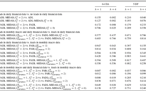
Table 4. Testing for equal predictive ability for models with leads
64 DA 5 DF
h=1 h=4 h=1 h=4
Leads in daily financial data vs. no leads in daily financial data ADL-MIDAS(JD
X =2) vs. ADL 0.155 0.002 0.210 0.040
ADL-MIDAS(JD
X =2) vs. ADL-MIDAS(J D
X =0) 0.127 0.002 0.193 0.076
FADL-MIDAS(JD
X =2) vs. FADL 0.172 0.008 0.179 0.233
FADL-MIDAS(JD
X =2) vs. FADL-MIDAS(JXD=0) 0.706 0.025 0.209 0.358
Leads in monthly macro and daily financial data vs. leads in daily financial data FADL-MIDAS(JM
CFNAI=1, JXD=2) vs. FADL-MIDAS(JXD=2) 0.377 0.437 0.671 0.786
FADL-MIDAS(JM
NAPMNOI=2, J
D
X =2) vs. FADL-MIDAS(J D
X =2) 0.403 0.766 0.759 0.814
Leads in daily financial data vs. leads in monthly macro data FADL-MIDAS(JD
X =2) vs. FAR(JCFNAIM =1) 0.947 0.043 0.397 0.155
FADL-MIDAS(JD
X =2) vs. FAR(J M
NAPMNOI=2) 0.814 0.034 0.608 0.164
FADL-MIDAS(JD
X =2) vs. FADL(J M
CFNAI=1) 0.504 0.358 0.936 0.345
FADL-MIDAS(JD
X =2) vs. FADL(J M
NAPMNOI=1) 0.420 0.386 0.903 0.441
FADL-MIDAS(JD
X =2) vs. FADL-MIDAS(J M
CFNAI=1, J
D
X =0) 0.394 0.509 0.817 0.487
FADL-MIDAS(JD
X =2) vs. FADL-MIDAS(JNAPMNOIM =2, JXD=0) 0.350 0.556 0.882 0.258
Leads in monthly macro and daily financial data vs. leads in monthly macro data FADL-MIDAS(JM
CFNAI=1, J
D
X =2) vs. FAR(J M
CFNAI=1) 0.007 0.002 0.037 0.086
FADL-MIDAS(JM
NAPMNOI=2, JXD=2) vs. FAR(JNAPMNOIM =2) 0.012 0.006 0.196 0.099
FADL-MIDAS(JM
CFNAI=1, JXD=2) vs. FADL(JCFNAIM =1) 0.008 0.019 0.205 0.210
FADL-MIDAS(JM
NAPMNOI=2, JXD=2) vs. FADL(J M
NAPMNOI=2) 0.838 0.071 0.676 0.414
FADL-MIDAS(JM
CFNAI=1, JXD=2) vs. FADL-MIDAS(JCFNAIM =1, JXD=0) 0.649 0.028 0.629 0.324
FADL-MIDAS(JM
NAPMNOI=2, J
D
X =2) vs. FADL-MIDAS(J M
NAPMNOI=2, J
D
X =0) 0.138 0.727 0.731 0.240
NOTE: This table reportsp-values of the two-sided hypotheses that compare the predictive ability between selected families of models reported inTable 3. All comparisons are based on the Diebold–Mariano test.
defined as follows: the macroeconomic predictor in quartert+1 andJM
X =1,2 monthly leads.
Notice that the parsimony of the above specification reflects the limited number of degrees of freedom. Specifically, Equa-tion (5.1) incorporates the macroeconomic information through lags of quarterly macroeconomic factors and leads of individual macroeconomic indicators at the monthly frequency. This means that, compared with the FADL-MIDAS(JXD=2) model, the
FADL-MIDAS(JCFNAIM =1, JXD =2) model has only one
addi-tional parameter and the FADL-MIDAS(JNAPMNOIM =2, JXD =
2) model has two extra parameters to estimate. While this spec-ification restricts the form of macroeconomic information that enters into the model (e.g., uses lags of quarterly macroeco-nomic data rather than monthly data if available), it is an appeal-ing way to generalize the current nowcastappeal-ing literature, which largely ignores the daily financial information.
A notable exception is the study by Banbura et al. (2012) who employed a dynamic factor state-space model for nowcast-ing the U.S. GDP growth and unlike the previous literature, they used daily and weekly financial variables in addition to macroe-conomic variables available at a monthly frequency. Beyond the methodological differences between MIDAS regression with leads and the dynamic factor state-space model discussed in Section2.2, our study differs from their contribution in one im-portant aspect. While we emphasize the importance of the daily financial data by employing a rather large cross-section of daily financial data, they only used a handful of daily financial assets. Hence, our results are not directly comparable.
Similarly, we can obtain the third family of models that use leads in monthly macroeconomic data but ignore the real-time information of the daily financial variables. These models can be viewed as generalizations of the traditional FAR and FADL models as well as the FADL-MIDAS(JD
X =0) model to include leads in monthly macroeconomic data.
We find that both FADL-MIDAS(JCFNAIM =1, JXD =2) and
FADL-MIDAS(JNAPMNOIM =2, JXD =2) exhibit similar
predic-tive ability to models with leads in daily financial data alone (FADL-MIDAS(JXD =2)). Table 4 shows that we accept the
null of equal predictive ability between models with leads in both monthly macroeconomic data and daily financial data against models with leads only in financial data. A similar finding holds for the comparison with models that only use
leads in macroeconomic data as long as one uses the FADL-MIDAS(JM
CFNAI=1, JXD =0) or FADL-MIDAS(JNAPMNOIM = 2, JD
X =0) models. Interestingly, the FADL-MIDAS models that use leads in both monthly macroeconomic data and daily financial data outperform models that ignore the daily finan-cial data and use the traditional FAR or FADL with leads in monthly macroeconomic data. In particular, we find that we reject the null of equal predictive ability between the two families of models, especially for the case of 64 daily assets (64 DA).
Furthermore, a closer inspection of the models with leads in only monthly macro reveals the following three observa-tions. First, we find that the FADL and FADL-MIDAS models with monthly leads in CFNAI or NAPMNOI outperform the corresponding FAR models. Second, the extra month of infor-mation in models that use leads in NAPMNOI does not provide substantial forecasting gains over models that use 1 month of leads in CFNAI. Third, an RMSFE comparison between FADL-MIDAS(JXD=2) and FADL-MIDAS(JNAPMNOIM =2, JXD =0)
yields a mixed picture, which depends on the forecasting hori-zon, at least for the long sample. Nevertheless, we accept the null of equal predictive ability between the two families of models for both forecasting horizons.
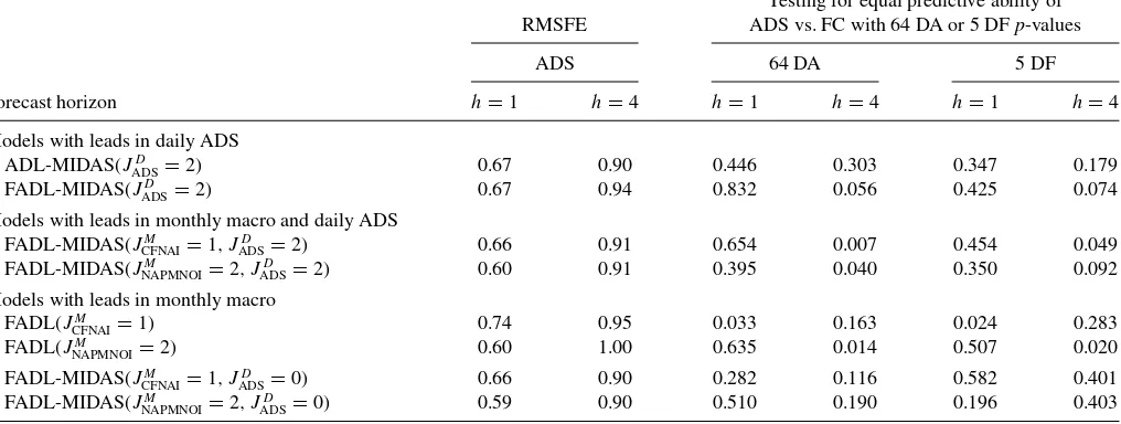
While we established that the MIDAS regression models that use leads in daily financial data have similar forecasting ability with the MIDAS regression models that use leads in monthly macroeconomic data, one concern remains. Can models that use leads in daily macroeconomic data outperform models that use leads in daily financial data? To answer this question, we estimate models with leads in ADS data for the long sample and report their RMSFE forh=1,4 inTable 5. We also compare their predictive ability with forecast combinations of models with 64 DA and 5 DF in Tables 1 and3. We find that while for all families of models, MIDAS regression models with ADS perform better than the corresponding forecast combinations of daily assets or factors, in general, we accept the null of equal predictive ability.
Moreover, similar findings are also obtained when we replace the 2 months of leads in NAPMNOI with 2 months of leads in the Total Nonfarm Payroll Employment (EMPLOY). A notable difference is that the forecasting gains for all families of models are generally weaker than the results for CFNAI and NAPMNOI. These results are only reported in the Internet Appendix to save space.
A final point is that the gains of MIDAS regression models with leads naturally generate the question of which class of fi-nancial assets is the most salient. In general, we find that there is no dominant class for the whole sample but rather the forecast combination weights for all five classes are generally stable. Some instability is observed toward the end of the sample due to the financial crisis, but it is rather moderate and ambiguous, as it occurs at the end of the sample. In particular, while rela-tively more weight is placed on equities until the beginning of the financial crisis, the role of corporate risk and government securities becomes more important at the beginning of the fi-nancial crisis. More details on the classes of assets can be found in the Internet Appendix where we report time-plots of forecast combination weights as well as a table of best predictors for both long and short samples.
Table 5. Comparisons with ADS
Testing for equal predictive ability of RMSFE ADS vs. FC with 64 DA or 5 DFp-values
ADS 64 DA 5 DF
Forecast horizon h=1 h=4 h=1 h=4 h=1 h=4
Models with leads in daily ADS ADL-MIDAS(JD
ADS=2) 0.67 0.90 0.446 0.303 0.347 0.179
FADL-MIDAS(JD
ADS=2) 0.67 0.94 0.832 0.056 0.425 0.074
Models with leads in monthly macro and daily ADS FADL-MIDAS(JM
CFNAI=1, JADSD =2) 0.66 0.91 0.654 0.007 0.454 0.049
FADL-MIDAS(JM
NAPMNOI=2, J
D
ADS=2) 0.60 0.91 0.395 0.040 0.350 0.092
Models with leads in monthly macro FADL(JM
CFNAI=1) 0.74 0.95 0.033 0.163 0.024 0.283
FADL(JM
NAPMNOI=2) 0.60 1.00 0.635 0.014 0.507 0.020
FADL-MIDAS(JM
CFNAI=1, J
D
ADS=0) 0.66 0.90 0.282 0.116 0.582 0.401
FADL-MIDAS(JM
NAPMNOI=2, JADSD =0) 0.59 0.90 0.510 0.190 0.196 0.403
NOTE: The first two columns of the table present pseudo out-of-sample RMSFEs using MIDAS regression models that replace the daily financial asset with the ADS variable. The remaining four columns presentp-values of two-sided hypotheses that compare the models with ADS against the corresponding models based on forecast combinations (FC) of 64 daily assets (64 DA) or 5 daily factors (5 DF) inTable 3. All comparisons are based on the Diebold–Mariano test.
6. CONCLUSION
We study MIDAS regression models that are capable of incor-porating forward-looking information in daily financial assets or factors to provide direct out-of-sample forecasts of U.S. quar-terly real GDP growth. In doing so, we take advantage of the data-rich financial environment by constructing a comprehen-sive dataset of around 1000 daily financial predictors that span the five major classes of assets: corporate risk, equities, fixed income, commodities, and foreign exchange. We propose two complementary approaches to deal with the large cross-section of daily series. The first extracts daily financial factors and the second uses forecast combination methods of MIDAS regres-sion models with daily financial assets or factors.
Overall, our findings emphasize the role of reduced-form MI-DAS regressions in exploiting the daily financial information for forecasting the quarterly real GDP growth. We find that MIDAS regression models using daily financial information via daily financial assets or factors improve quarterly forecasts of U.S. real GDP growth beyond the quarterly macroeconomic factors. Furthermore, MIDAS regression models with leads offer an easy to implement reduced-form alternative method that can produce direct multistep horizon predictions compared with the typical nowcasting involving parameter-rich state-space model that produce current quarter and possiblyh-step ahead iterated forecasts. More importantly, MIDAS regression models with leads provide a parsimonious approach to deal with a large cross-section of high-frequency predictors. Traditional nowcasting only deals with the very detailed calendar of macroeconomic releases and involves state-space models potentially involving many (measurement) equations and lots of parameters especially for a large set of daily financial predictors. When we compare MIDAS models with leads in both monthly macroeconomic data and daily financial data, we find that these models exhibit similar predictive ability to models with leads in daily financial data alone. However, the forecasting ability of models that ignore the daily financial information in favor of aggregate financial data
and monthly macro leads can have relatively inferior forecasting performance. In this sense, it appears that MIDAS regression models with leads are able to take advantage of the financial data-rich environment both in terms of the higher frequency of the data and the large cross-section of financial predictors.
Finally, forecasting real GDP growth is only one of many ex-amples where our methods can be applied. The generic question we addressed is how one can use large panels of high-frequency data to improve forecasts of low-frequency series. There are many other macroeconomic series to which this can be applied as well as many other applications in economics and other fields where this problem occurs. Our methods are therefore of gen-eral interest beyond the specific application considered in the present article.
ACKNOWLEDGMENTS
Elena Andreou acknowledges support of the European Research Council under the European Community FP7/2008-2013 ERC grant 209116. Eric Ghysels acknowledges support of a Marie Curie FP7-PEOPLE-2010-IIF grant and benefited from funding by the Federal Reserve Bank of New York through the Resident Scholar Program. We also thank Tobias Adrian, Jennie Bai, Jushan Bai, Frank Diebold, Rob Engle, Ana Galv˜ao, Michael Fleming, Serena Ng, Simon Potter, Lucrezia Reichlin, Jim Stock, Mark W. Watson, Jonathan H. Wright, and Michael McCracken as well as seminar participants at the Banque de France, Banca d’Italia, Board of Governors of the Federal Reserve, Columbia University, Deutsch Bundesbank, Federal Reserve Bank of New York, HEC Lausanne, Queen Mary University, the University of Pennsylvania, the University of Chicago, the CIRANO/CIREQ Financial Econometrics Conference, the Midwest Economet-rics Group Conference, the Econometric Society European Meeting, the EC2 Conference—Aarhus, the NBER Summer Institute, the NBER/NSF Time Series Conference at Duke
University, the Royal Economic Society conference, and the 6th European Central Bank Workshop on Forecasting Techniques for comments at various versions of this article. We also thank Constantinos Kourouyiannis, Michael Sockin, Athanasia Petsa, and Elena Pilavaki for providing excellent research assistance on various parts of the article. Last but not least we thank the Editor, an associate editor, and two anonymous referees for their helpful comments.
[Received January 2012. Revised December 2012.]
REFERENCES
Aiolfi, M., and Timmermann, A. (2006), “Persistence in Forecasting Perfor-mance and Conditional Combination Strategies,”Journal of Econometrics, 135, 31–53. [245]
Andreou, E., Ghysels, E., and Kourtellos, A. (2011), “Forecasting With Mixed-Frequency Data,” inOxford Handbook of Economic Forecasting, eds. M. Clements and D. Hendry, Oxford University Press. [240]
——— (2012), “Internet Appendix: Should Macroeconomic Fore-casters Use Daily Financial Data and How?” Available at http://www.unc.edu/eghysels/working_papers.html. [242]
Armesto, M. T., Engemann, K. M., and Owyang, M. T. (2010), “Forecasting With Mixed Frequencies,”Federal Reserve Bank of St. Louis Review, 92, 521–536. [240]
Armesto, M. T., Hernandez-Murillo, R., Owyang, M., and Piger, J. (2009), “Measuring the Information Content of the Beige Book: A Mixed Data Sampling Approach,”Journal of Money, Credit and Banking, 41, 35–55. [240]
Aruoba, S. B., Diebold, F. X., and Scotti, C. (2009), “Real-Time Measurement of Business Conditions,”Journal of Business and Economic Statistics, 27, 417–427. [241,243]
Bai, J. (2003), “Inferential Theory for Factor Models of Large Dimensions,” Econometrica, 71, 135–171. [244]
Bai, J., Ghysels, E., and Wright, J. (2010), “State Space Models and MIDAS Regressions,”Econometric Reviews(forthcoming). [241,245]
Bai, J., and Ng, S. (2002), “Determining the Number of Factors in Approximate Factor Models,”Econometrica, 70, 191–221. [244]
Banbura, M., Giannone, D., Modugno, M., and Reichlin, L. (2012), “Now-Casting and the Real-Time Data,” inHandbook of Economic Forecasting (Vol. 2), eds. G. Elliott and A. Timmermann, Amsterdam: Elsevier-North Holland (forthcoming). [249]
Buchmann, M. (2011), “Corporate Bond Spreads and Real Activity in the Euro Area—Least Angle Regression Forecasting and the Probability of the Re-cession,” ECB Working Paper, Frankfurt: European Central Bank. [243] Clark, T. E., and McCracken, M. W. (2012), “Advances in Forecast
Evalua-tion,” inHandbook of Economic Forecasting(Vol. 2), eds. G. Elliott and A. Timmermann, Amsterdam: Elsevier-NorthHolland (forthcoming). [247] Clements, M. P., and Galv˜ao, A. B. (2008), “Macroeconomic Forecasting With
Mixed Frequency Data: Forecasting US Output Growth,”Journal of Busi-ness and Economic Statistics, 26, 546–554. [240,242]
——— (2009), “Forecasting US Output Growth Using Leading Indicators: An Appraisal Using MIDAS Models,”Journal of Applied Econometrics, 24, 1187–1206. [240]
D’Agostino, A., Surico, P., and Giannone, D. (2007), “(Un)Predictability and Macroeconomic Stability,” CEPR Discussion Paper, London: Centre of Eco-nomic Policy Research. [243]
Diebold, F. X., and Mariano, R. S. (1995), “Comparing Predictive Accuracy,” Journal of Business and Economic Statistics, 13, 253–265. [246] Edelstein, P. (2007), “Commodity Prices, Inflation Forecasts and Monetary
policy,” Working Paper, Ann Arbor, MI: University of Michigan. [243] Forni, M., Hallin, M., Lippi, M., and Reichlin, L. (2000), “The Generalized
Dynamic-Factor Model: Identification and Estimation,”Review of Eco-nomics and Statistics, 82, 540–554. [244]
——— (2005), “The Generalized Dynamic Factor Model,”Journal of the American Statistical Association, 100, 830–840. [244]
Foroni, C., Marcellino, M., and Schumacher, C. (2011), “U-MIDAS: MI-DAS Regressions With Unrestricted Lag Polynomials,” Discussion Paper, Deutsche Bundesbank and European University Institute. [241]
Frale, C., Marcellino, M., Mazzi, G. L., and Proietti, T. (2011), “EUROMIND: A Monthly Indicator of the Euro Area Economic Conditions,”Journal of the Royal Statistical Society,Series A, 174, 439–470. [240]
Ghysels, E., Sinko, A., and Valkanov, R. (2006), “MIDAS Regres-sions: Further Results and New Directions,” Econometric Reviews, 26, 53–90. [241]
Ghysels, E., and Valkanov, R. (2012), “Forecasting Volatility With MIDAS,” in Handbook of Volatility Models and Their Applications, eds. L. Bauwens, C. Hafner, and S. Laurent, Hoboken, NJ: Wiley, pp. 383–401. [240] Ghysels, E., and Wright, J. (2009), “Forecasting Professional Forecasters,”
Jour-nal of Business and Economic Statistics, 27, 504–516. [240,242] Giannone, D., Reichlin, L., and Small, D. (2008), “Nowcasting: The
Real-Time Informational Content of Macroeconomic Data,”Journal of Monetary Economics, 55, 665–676. [242]
G¨urkaynak, R. S., Sack, B., and Wright, J. (2010), “The Tips Yield Curve and Inflation Compensation,”American Economics Journal: Macroeconomics, 2, 70–92. [243]
Hamilton, J. D. (2008), “Daily Monetary Policy Shocks and New Home Sales,” Journal of Monetary Economics, 55, 1171–1190. [240]
Harvey, D. I., Leybourne, S. J., and Newbold, P. (1997), “Testing the Equality of Prediction Mean Squared Errors,”International Journal of Forecasting, 13, 281–291. [247]
Hendry, D. F., and Clements, M. P. (2004), “Pooling of Forecasts,”Econometrics Journal, 7, 1–131. [245]
Kuzin, V., Marcellino, M., and Schumacher, C. (2011), “MIDAS Versus Mixed-Frequency VAR: Nowcasting GDP in the Euro Area,”International Journal of Forecasting, 27, 529–542. [240]
——— (2012), “Pooling Versus Model Selection for Nowcasting GDP With Many Predictors: Empirical Evidence for Six Industrialized Countries,” Journal of Applied Econometrics, forthcoming. [240,242]
Ludvigson, S., and Ng, S. (2007), “The Empirical Risk-Return Relation: A Factor Analysis Approach,” Journal of Financial Economics, 83, 171– 222. [244]
——— (2009), “Macro Factors in Bond Risk Premia,”Review of Financial Studies, 12, 5027–5067. [244]
Marcellino, M., Stock, J. H., and Watson, M. W. (2006), “A Comparison of Direct and Iterated Multistep ar Methods for Forecasting Macroeconomic Time Series,”Journal of Econometrics, 135, 499–526. [242]
Monteforte, L., and Moretti, G. (2013), “Real Time Forecasts of Inflation: The Role of Financial Variables,” Journal of Forecasting, 32, 51–61. [240]
Nunes, L. C. (2005), “Nowcasting Quarterly gdp Growth in a Monthly Coinci-dent Indicator Model,”Journal of Forecasting, 24, 575–592. [242] Schumacher, C., and Breitung, J. (2008), “Real-Time Forecasting of German
GDP Based on a Large Factor Model With Monthly and Quarterly Data,” International Journal of Forecasting, 24, 386–398. [240]
Stock, J. H., and Watson, M. W. (1989), “New Indexes of Coincident and Leading Economic Indicators,” inNBER Macroeconomics Annual(Vol. 4), eds. O. J. Blanchard and S. Fischer, Cambridge, MA: MIT Press, pp. 351– 394. [244]
——— (2002a), “Forecasting Using Principal Components From a Large Num-ber of Predictors,”Journal of the American Statistical Association, 97, 1167– 1179. [244]
——— (2002b), “Macroeconomic Forecasting Using Diffusion Indexes,” Jour-nal of Business and Economic Statistics, 20, 147–162. [244,245,247] ——— (2003), “Forecasting Output and Inflation: The Role of Asset Prices,”
Journal of Economic Literature, 41, 788–829. [241,244,245]
——— (2004), “Combination Forecasts of Output Growth in a Seven-Country Data Set,”Journal of Forecasting, 23, 405–430. [245]
——— (2006), “Macroeconomic Forecasting Using Many Predictors,” in Handbook of Economic Forecasting, eds. G. Elliott, C. Granger, and A. Timmermann, Amsterdam: Elsevier-North Holland, pp. 87–115. [244] ——— (2008a), “Forecasting in Dynamic Factor Models Subject to Structural
Instability,” inThe Methodology and Practice of Econometrics, A Festschrift in Honour of Professor David F. Hendry, eds. Jennifer Castle and Neil Shephard, Oxford: Oxford University Press. [244]
——— (2008b), “Phillips Curve Inflation Forecasts,” NBER Working Paper, Cambridge, MA: National Bureau of Economic Research. [243,244,245] Timmermann, A. (2006), “Forecast Combinations,” inHandbook of Economic
Forecasting (Vol. 1), eds. G. Elliott, C. Granger, and A. Timmermann, Amsterdam: Elsevier-North Holland, pp. 136–196. [245]
West, K. D. (1996), “Asymptotic Inference About Predictive Ability,” Econo-metrica, 64, 1067–1084. [246]