Full Terms & Conditions of access and use can be found at
http://www.tandfonline.com/action/journalInformation?journalCode=ubes20
Download by: [Universitas Maritim Raja Ali Haji], [UNIVERSITAS MARITIM RAJA ALI HAJI
TANJUNGPINANG, KEPULAUAN RIAU] Date: 11 January 2016, At: 20:41
Journal of Business & Economic Statistics
ISSN: 0735-0015 (Print) 1537-2707 (Online) Journal homepage: http://www.tandfonline.com/loi/ubes20
Comment
Elena Andreou & Eric Ghysels
To cite this article: Elena Andreou & Eric Ghysels (2014) Comment, Journal of Business & Economic Statistics, 32:2, 168-171, DOI: 10.1080/07350015.2014.902238
To link to this article: http://dx.doi.org/10.1080/07350015.2014.902238
Published online: 16 May 2014.
Submit your article to this journal
Article views: 125
View related articles
168 Journal of Business & Economic Statistics, April 2014
Comment
Elena A
NDREOUDepartment of Economics, University of Cyprus, P.O. Box 537, CY 1678 Nicosia, Cyprus ([email protected])
Eric G
HYSELSDepartment of Economics, University of North Carolina, Gardner Hall CB 3305, Chapel Hill, NC 27599; Department of Finance, Kenan-Flagler Business School, Chapel Hill, NC 27599 ([email protected])
1. INTRODUCTION
The article by Hu and Tsay (2013) relates to an important area of research on analyzing multivariate time series with dynamic heteroscedasticity and addresses the dimensionality problem of traditional multivariate models for financial asset returns volatil-ities via common factor analysis. This article provides an alter-native approach to estimate the common volatility factor for multivariate dynamic heteroscedastic processes. The principal volatility component (PVC) proposed is based on the cumula-tive generalized kurtosis matrix which summarizes the higher order dynamics of multivariate volatility processes. The spectral analysis decomposition of the cumulative generalized kurtosis matrix is used to estimate the PVC. Given that one of the factors may not have dynamic heteroscedasticity, a generalized test is proposed for the presence of no ARCH type dependence. Sim-ulation and empirical results provide additional evidence of the PVC procedure and test properties. Hu and Tsay (2013) worked on a fundamental question of extracting common volatility fac-tors which are especially relevant for financial time series. We are therefore pleased to contribute some comments related to the volatility factor estimation some of which are also addressed in our own related recent work (Andreou and Ghysels 2013; Ghysels2013).
The idea to estimate the common volatility factor from a cross-section of volatilities for financial time series is not new but has been in an area of recent research. Early contributions in the common volatility factor analysis involving small cross-sections of assets includes various ARCH factor models, see, for example, Engle (1987); Engle, Ng, and Rothschild (1990); and Ng, Engle, and Rothschild (1992), among others. Diebold and Nerlove (1989) suggested a closely related latent factor model. For larger cross-sections of financial returns with dynamic het-eroscedasticity, Connor, Korajczyk, and Linton (2006) devel-oped a dynamic approximate factor model and relied on large panel data asymptotics to estimate a common volatility com-ponent. Their analysis involves a semiparametric ARCH-type volatility filter. Instead, Anderson and Vahid-Araghi (2007) and Barigozzi et al. (2013) used large panels of realized volatilities to extract the common volatility factor. In the context of risk neu-tral pricing there are also examples of factor analysis. B¨uhler (2006), Amengual (2009), Egloff, Leippold, and Wu (2010), and A¨ıt-Sahalia, Karaman, and Mancini (2012) applied princi-pal component analysis (PCA) to panels of variance swap rates and found that two factors—which can be interpreted as level and slope—explain close to 100% of the variation in variance swap rates for the S&P 500.
In view of some of the above literature, we first briefly de-scribe the PVC estimation approach in Hu and Tsay (2013) in the next section. In the following section, we revisit their simulation design to evaluate the role of the finite higher order moment condition in their PVC procedure. In the last section, we discuss some further results on common volatility factor es-timation which are related to our recent work and complement the results of Hu and Tsay (2013).
2. THE PRINCIPAL VOLATILITY COMPONENT (PVC)
PROCEDURE
Let the multivariate stochastic processyt beα-mixing such as for instance an ARCH-type process. Hu and Tsay (2013) as-sumed thatyt is ak-dimensional weakly stationary time series with finite fourth moments. Hence, the generalized kurtosis ma-trixγl ofyt captures the dynamics of the fourth power ofyty′t wherexij,t−lcan be, for example, the Huber’s function
xij,t−l= eralized covariance matrix and the cumulative matrix is given by: Journal of Business & Economic Statistics
April 2014, Vol. 32, No. 2 DOI:10.1080/07350015.2014.902238
such that Ŵˆm =Ŵm+O(1/√n) assuming yt has finite sixth moments.
The idea of the common volatility factor or more precisely the PVC in Hu and Tsay (2013) is based on the spectral analysis of the generalized kurtosis matrix of the multivariate observed financial processes,Ŵˆm in (4). The novel aspect of the Hu and Tsay (2013) procedure compared to the papers mentioned in the Introduction is related to the generalized kurtosis matrix estimation and the principal component estimation based on this matrix. One advantage of this procedure is that it is based on the observed process,yt. Yet the squared cross-products of ytinvolved inγlcan be noisy estimates of volatility. This point is discussed further in the last section given it relates to an alternative approach to estimate common volatility factors.
3. PVC AND FINITE MOMENT CONDITIONS
The objective of this section is to examine the finiteness of the higher moments condition required in the PVC theory of Hu and Tsay (2013). Examples of such financial processes where the fourth moments are not finite are empirically relevant for fi-nancial time series such as weekly processes (as presented in the empirical analysis of the article) as well as higher frequencies. ARCH-type models with highly leptokurtic distributions or the Integrated GARCH (IGARCH) model are found in empirical research. Although Hu and Tsay (2013) provided simulation results for highly persistent normal ARCH models that do not satisfy the finite fourth moment condition we present additional simulation evidence in this section.
First, we follow the simulation design in Hu and Tsay (2013) and extend it to study the performance of the PVC in vari-ous other cases where the individual ARCH-type processes,ft defined below, do not necessarily satisfy the conditions of finite-ness of higher order moments in ARCH-type processes. In their Monte Carlo design, Hu and Tsay (2013) assumed that the mul-tivariate factor structure is driven by mulmul-tivariate normal errors. Therefore, in the second step we extend the simulation results to the case where the multivariate ARCH-type processes are driven by highly leptokurtic error distributions and reexamine the PVC procedure.
We simulate the following data-generating processes (DGPs) to further examine the performance of the PVC when the mo-ments of the ARCH-type processes are not finite following mod-elsft=σtet where we first assume that volatility follows an integrated GARCH model:
σt2=ω+αft2−1+βσt2−1, (5)
with α+β =1. Second, we assume the ARCH models are driven by Student’s-terrors,et, with 3 and 5 degrees of freedom1
σt2=ω+αft2−1. (6)
Third, we consider the GJR-ARCH model
σt2 =ω+αft2−1+βσt2−1+τft2−1It−1, (7)
1It is worth noting that we used the standardized Student’s-tdistribution for the
t-ARCH DGP (Bollerslev and Engle1986) which is not the same as that in the
build-in ARCH routine in Matlab that uses unstandardized Student’s-terrors.
with high persistence and normal or t(3) errors whereτ is the threshold parameter and It−1=0 ifet−1≥0, andIt−1=1 if et−1<0. Finally, we consider an AR-ARCH model
ft =ρft−1+σtet, σt2 =ω+αf
2
t−1 (8)
whereρis set to be equal to 0.1 or 0.9 withet ∼normal. In the AR-ARCH model, we consider bothftandftin our analysis. Note that for completeness we also simulate the high persistence (HP) Normal ARCH models as given in Hu and Tsay (2013) as well as the corresponding low-persistence (LP) normal ARCH for which the finite fourth moment conditions are satisfied.
The multivariate ARCH factor model is given by
yt=Hft+ǫt, (9)
where H is the k×r loading matrix, ft=(f1t, . . . , frt) are independent conditional heteroscedastic processes andǫtis the
k×T noise term, a sequence of independent and identically dis-tributed random vectors with zero mean and constant positive-definite covariance matrixt. In the first step, we assumeǫt follows a normal distribution as in Hu and Tsay (2013) and ft is either of the ARCH-type models in (5)–(8). These results are reported in Table 1. In the second step, we assumeǫt fol-lows at(3) distribution and report the corresponding results in Table 2.
Table 1reports the results for the correlations coefficientsR1 andR2given by 5 for the Huber’s function follows from the relatively good performance of the simulation results reported in Hu and Tsay (2013). The case ofm=10 was also applied in the simulations and gave similar results.
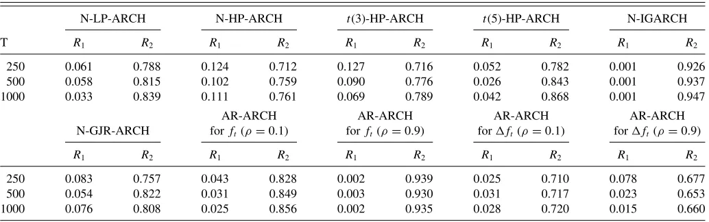
The general conclusion from the results reported inTable 1is that even if the ARCH-type processes inft do not satisfy the fi-nite fourth moment conditions, the PVC behaves well according to criteriaR1andR2which are expected to be close to zero and one, respectively. Hence, our results inTable 1provide further support in favor of the simulation evidence presented in Hu and Tsay (2013) for different DGPs.Table 2reports the results for some of the ARCH processes inftas above, but nowǫtin Equa-tion (9) follows the standardized Student’st-(3) distribution. In contrast to the results in Table 1, those in Table 2 show that the PVC performs relatively less well when the noise term is t(3) distributed. In particular, theR2criterion falls and theR1 criterion increases especially for both the normal and Student’s-t(3) high-persistent ARCH-type models,ft. This result is valid even for large samplesT for the highly persistent ARCH mod-els. Therefore extending the simulation analysis of Hu and Tsay (2013), we find that there are cases especially when the error distribution of the multivariate factor ARCH model in (9) is highly leptokurtic that the relative performance of the PVC, via the measuresR1andR2, is weaker compared to the case where ǫt is normal. It is also worth noting that the results on PVC become worse whenǫt in Equation (9) follows an asymmetric distribution such as the log–normal.
170 Journal of Business & Economic Statistics, April 2014
Table 1. Principal volatility component analysis summary statistics,yt =Hft+ǫt,ǫt ∼N(0,1)
N-LP-ARCH N-HP-ARCH t(3)-HP-ARCH t(5)-HP-ARCH N-IGARCH
T R1 R2 R1 R2 R1 R2 R1 R2 R1 R2
250 0.033 0.890 0.037 0.839 0.080 0.795 0.046 0.831 0.0004 0.924
500 0.019 0.932 0.019 0.889 0.075 0.824 0.041 0.857 0.0003 0.938
1000 0.011 0.954 0.050 0.839 0.052 0.839 0.037 0.889 0.0003 0.942
AR-ARCH AR-ARCH AR-ARCH AR-ARCH
N-GJR-ARCH forft (ρ=0.1) forft(ρ=0.9) forft (ρ=0.1) forft(ρ=0.9)
R1 R2 R1 R2 R1 R2 R1 R2 R1 R2
250 0.030 0.842 0.026 0.856 0.023 0.944 0.040 0.631 0.052 0.663
500 0.032 0.845 0.024 0.860 0.002 0.949 0.026 0.668 0.073 0.650
1000 0.011 0.954 0.023 0.870 0.002 0.955 0.028 0.628 0.062 0.654
NOTES: The table shows the summary statistics of the Hu and Tsay (2013) principal volatility component analysis for variousk=five-dimensional series forft. The multivariate factor ARCH model is given by Equation (5) whereǫt∼N(0,1). The performance measuresR1andR2in (10) are calculated using 1000 iterations in Matlab. For theŴˆmmatrixm=5 is
used and for the Huber’s functionc=2.5. We used Hu and Tsay (2013) high-persistent HP-ARCH components for all the ARCH, GJR-ARCH and AR-ARCH models, that is (ω,α)
=(1,0.9), (2,0.8), (3,0.7), and (1,0.95). For the low-persistent LP-ARCH models the ARCH parameter of the 4 ARCH(1) components areα=0.1,0.2,0.3,0.4, respectively. In the IGARCH model, (ω,α,β)=(1,0.09,0.9), (2,0.06,0.93), (3,0.05,0.94), (1,0.02,0.97).N,t(3), andt(5) denote the standard normal and the standardized Student’st-(3) and Student’st-(5) innovation’s distribution.ρis the AR coefficient of the AR(1)–ARCH(1) models.
4. AN ALTERNATIVE APPROACH FOR COMMON
VOLATILITY FACTOR ESTIMATION
The analysis of Hu and Tsay (2013) does not address certain aspects of common volatility factor estimation namely the large cross-sectional dimension, the alternative volatility filters and the use of high-frequency data, as well as the selection of the number of volatility factors.
These aspects are addressed in our recent work (Andreou and Ghysels2013; Ghysels2013). We provide the asymptotic analy-sis of common volatility risk factor estimation using large panels of filtered volatilities such as (1) parametric spot volatility filters (e.g., ARCH-type models) or (2) data-driven realized volatili-ties (e.g., Zhang 2001; Andreou and Ghysels2002; Mykland and Zhang2008) and data-driven spot volatilities (e.g., Zhang, Mykland and A¨ıt-Sahalia2005; Hansen and Lunde2006). Un-like Hu and Tsay (2013), who consider the cumulative gener-alized kurtosis matrix based on cross-products of yt, we
esti-mate common volatility factors directly from panels of filtered volatilities. Specifically we consider the following model rep-resentation forX[h:t] =( ˆV[ih:t], i=1, . . . , N)′, where ˆV
i
[h:t] are the filtered volatilities. LetF0
t be ther×1 vector of the true population volatility factors with either:Ft0 = σ(Xtf)2,when panels of spot volatilities are consider, andFt0=tt−dσ(Xτf)2dτ with integrated volatility proxies, whereXtf are the latent fac-tors of a continuous time affine diffusion model. Moreover, for factor loadings0= (λ01, . . . , λ0N)′,we have the following factor
representation:
X[h:t]=0Ft0+e[h:t], (11) wheree[h:t] =(e[ih:t], i=1, . . . , N)′.We use principal compo-nent analysis with panels of filtered volatilities.
The common volatility factor estimation analysis is based on three types of asymptotic expansions: the cross-section of volatility estimates at each point in time, that isi=1, . . . , N
Table 2. Principal volatility component analysis summary statistics,yt =Hft+ǫt,ǫt∼t(3)
N-LP-ARCH N-HP-ARCH t(3)-HP-ARCH t(5)-HP-ARCH N-IGARCH
T R1 R2 R1 R2 R1 R2 R1 R2 R1 R2
250 0.061 0.788 0.124 0.712 0.127 0.716 0.052 0.782 0.001 0.926
500 0.058 0.815 0.102 0.759 0.090 0.776 0.026 0.843 0.001 0.937
1000 0.033 0.839 0.111 0.761 0.069 0.789 0.042 0.868 0.001 0.947
AR-ARCH AR-ARCH AR-ARCH AR-ARCH
N-GJR-ARCH forft(ρ=0.1) forft(ρ=0.9) forft (ρ=0.1) forft(ρ=0.9)
R1 R2 R1 R2 R1 R2 R1 R2 R1 R2
250 0.083 0.757 0.043 0.828 0.002 0.939 0.025 0.710 0.078 0.677
500 0.054 0.822 0.031 0.849 0.003 0.930 0.031 0.717 0.023 0.653
1000 0.076 0.808 0.025 0.856 0.002 0.935 0.028 0.720 0.015 0.660
NOTES: The table shows the summary statistics of the Hu and Tsay (2013) principal volatility component analysis for variousk=five-dimensional series forft. The multivariate factor ARCH model is given by Equation (5) whereǫt∼t(3). The performance measuresR1andR2in (10) are calculated using 1000 iterations in Matlab. For theŴˆmmatrixm=5 is used and
for the Huber’s functionc=2.5. We used Hu and Tsay (2013) high-persistent HP-ARCH components for all the models, that is (ω,α)=(1,0.9), (2,0.8), (3,0.7), and (1,0.95). For the low persistent LP-ARCH models the ARCH parameter of the 4 ARCH(1) components areα=0.1,0.2,0.3,0.4, respectively. In the IGARCH model, (ω,α,β)=(1,0.09,0.9), (2,0.06,0.93), (3,0.05,0.94), (1,0.02,0.97).N,t(3), andt(5) denote the standard normal and the standardized Student’s-t(3) and Student’s-t(5) innovation’s distribution.ρis the AR coefficient of the AR(1)–ARCH(1) models.
observed over a time spani=1, . . . , T and the sampling fre-quencyh of the data used to compute the volatility estimates which rely on data collected at increasing frequency,h↓0. The continuous record or in-fill asymptotics,h↓0, have a key role in that they can control the cross-sectional and serial correla-tion among the idiosyncratic errors of the panel of volatilities. Therefore under suitable regularity conditions, the traditional principal component analysis yields super-consistent estimates of the common volatility factors at each point in time. The in-tuition behind the super-consistency result is because the high-frequency sampling scheme of the filtered volatilities is tied to the size of the cross-section, boosting the rate of convergence. Consequently, the super-consistency of the common volatility factor extracted from the panel asymptotic arguments can also improve upon the individual volatility estimates.
In Hu and Tsay (2013), the analysis is based on the first PVC. An extension of the current analysis could address the choice of the number of factors. This question has been addressed in the context of linear factor models which do not involve common volatility factors (e.g., Stock and Watson2002; Bai and Ng2002). Namely, in the traditional factor models Bai and Ng (2002) among others proposed various information criteria that depend on the asymptotic rates ofN andT of the panel. In contrast, Ghysels (2013) showed that the standard cross-sectional criteria suffice for consistent estimation of the number of factors in large cross-sections of filtered volatilities, which is different from the traditional panel data results. This result on common volatility factor selection criteria draws from the super-consistency.
REFERENCES
A¨ıt-Sahalia, Y., Karaman, M., and Mancini, L. (2012), “The Term Structure of Variance Swaps, Risk Premia and the Expectation Hypothesis,” discussion
paper, Princeton University, Princeton, NJ. [168]
Amengual, D. (2009), “The Term Structure of Variance Risk Premia,” discussion
paper, Princeton University, Princeton, NJ. [168]
Anderson, H., and Vahid-Araghi, F. (2007), “Forecasting the Volatility of
Aus-tralian Stock Returns: Do Common Factors Help?,”Journal of Business and
Economic Statistics, 25, 76–90. [168]
Andreou, E., and Ghysels, E. (2002), “Rolling Sample Volatility Estimators:
Some New Theoretical, Simulation and Empirical Results,”Journal of
Busi-ness and Economic Statistics, 20, 363–376. [170]
——— (2013) “What Drives the VIX and the Volatility Risk Premium?”,
discussion paper, UCY and UNC. [168,170]
Bai, J., and Ng, S. (2002), “Determining the Number of Factors in Approximate
Factor Models,”Econometrica, 70, 191–221. [171]
Barigozzi, M., Brownlees, C. T., Gallo, G. M., and Veredas, D. (2013), “Disentangling Systematic and Idiosyncratic Dynamics in Panels of
Volatility Measures,” available at http://ssrn.com/abstract=1618565 or
http://dx.doi.org/10.2139/ssrn.1618565. [168]
Bollerslev, T., and Engle, R. F. (1986), “Modelling the Persistence of Conditional
Variances,”Econometric Reviews, 1, 1–50. [xxxx]
B¨uhler, H. (2006), “Consistent Variance Curve Models,”Finance and
Stochas-tics, 10, 178–203. [168]
Connor, G., Korajczyk, R. A., and Linton, O. (2006), “The Common and Specific
Components of Dynamic Volatility,”Journal of Econometrics, 132, 231–
255. [168]
Diebold, F. X., and Nerlove, M. (1989), “The Dynamics of Exchange Rate
Volatility: a Multivariate Latent Factor ARCH Model,”Journal of Applied
Econometrics, 4, 1–21. [168]
Egloff, D., Leippold, M., and Wu, L. (2010), “The Term Structure of Variance
Swap Rates and Optimal Variance Swap Investments,”Journal of Financial
and Quantitative Analysis, 45, 1279–1310. [168]
Engle, R. F. (1987), “Multivariate GARCH With Factor Structures— Cointegration in Variance,” unpublished manuscript, Department of
Eco-nomics, UCSD. [168]
Engle, R. F., Ng, V. K., and Rothschild, M. (1990), “Asset Pricing With a
Factor-ARCH Covariance Structure: Empirical Estimates for Treasury Bills,”
Jour-nal of Econometrics, 45, 213–237. [168]
Ghysels, E. (2013), “Factor Analysis With Large Panels of Volatility Proxies,”
discussion paper, UNC. [168,170,171]
Hansen, P. R., and Lunde, A. (2006), “Realized Variance and Market
Microstruc-ture Noise,”Journal of Business and Economic Statistics, 24, 127–161. [170]
Mykland, P. A., and Zhang, L. (2008), “Inference for Volatility-Type Objects
and Implications for Hedging,”Statistics and its Interface, 1, 255–278. [170]
Ng, V. K., Engle, R. F., and Rothschild, M. (1992), “A Multi-Dynamic-Factor
Model for Stock Returns,”Journal of Econometrics, 52, 245–266. [168]
Stock, J., and Watson, M. (2002), “Forecasting Using Principal Components
From a Large Number of Predictors,”Journal of the American Statistical
Association, 97, 1167–1179. [171]
Zhang, L. (2001), “From Martingales to ANOVA: Implied and Realized Volatil-ity,” Ph.D. thesis, Department of Statistics, University of Chicago, Chicago,
IL. [170]
Zhang, L., Mykland, P., and A¨ıt-Sahalia, Y. (2005), “A Tale of Two Time Scales:
Determining Integrated Volatility With Noisy High-Frequency Data,”
Jour-nal of the American Statistical Association, 100, 1394–1411. [170]
Comment
Juergen F
RANKEUniversit ¨at Kaiserslautern, Kaiserslautern, Germany ([email protected])
Financial data, in particular in the context of managing portfolios and quantifying their risk, come in the form of high-dimensional time series. The evolution of the coordinate processes, representing asset prices or returns, all depend on common market factors in addition to specific events concerning the value of the underlying asset only. An important task of financial time series analysis with major practical im-plications is the identification and description of such common factors.
In the present article, Hu and Tsay focus on the volatility aspect of financial time series and proposes an innovative way to structure the interdependencies between the fluctuations of the assets in a portfolio. For the volatility matrices, that is, the
© 2014American Statistical Association Journal of Business & Economic Statistics
April 2014, Vol. 32, No. 2 DOI:10.1080/07350015.2014.903652