Full Terms & Conditions of access and use can be found at
http://www.tandfonline.com/action/journalInformation?journalCode=ubes20
Download by: [Universitas Maritim Raja Ali Haji] Date: 11 January 2016, At: 22:51
Journal of Business & Economic Statistics
ISSN: 0735-0015 (Print) 1537-2707 (Online) Journal homepage: http://www.tandfonline.com/loi/ubes20
A Stochastic Volatility Model With Conditional
Skewness
Bruno Feunou & Roméo Tédongap
To cite this article: Bruno Feunou & Roméo Tédongap (2012) A Stochastic Volatility Model With Conditional Skewness, Journal of Business & Economic Statistics, 30:4, 576-591, DOI: 10.1080/07350015.2012.715958
To link to this article: http://dx.doi.org/10.1080/07350015.2012.715958
View supplementary material
Accepted author version posted online: 03 Aug 2012.
Submit your article to this journal
Article views: 447
A Stochastic Volatility Model With Conditional
Skewness
∗
Bruno F
EUNOUBank of Canada, Ottawa, Ontario, Canada K1A 0G9 ([email protected])
Rom ´eo T ´
EDONGAPStockholm School of Economics & Swedish House of Finance, SE-113 83 Stockholm, Sweden ([email protected])
We develop a discrete-time affine stochastic volatility model with time-varying conditional skewness (SVS). Importantly, we disentangle the dynamics of conditional volatility and conditional skewness in a coherent way. Our approach allows current asset returns to be asymmetric conditional on current factors and past information, which we term contemporaneous asymmetry. Conditional skewness is an explicit combination of the conditional leverage effect and contemporaneous asymmetry. We derive analytical formulas for various return moments that are used for generalized method of moments (GMM) estimation. Applying our approach to S&P500 index daily returns and option data, we show that one- and two-factor SVS models provide a better fit for both the historical and the risk-neutral distribution of returns, compared to existing affine generalized autoregressive conditional heteroscedasticity (GARCH), and stochastic volatility with jumps (SVJ) models. Our results are not due to an overparameterization of the model: the one-factor SVS models have the same number of parameters as their one-factor GARCH competitors and less than the SVJ benchmark.
KEY WORDS: Affine model; Conditional skewness; Discrete time; GMM; Option pricing.
1. INTRODUCTION
The option-pricing literature holds that generalized autoregressive conditional heteroscedasticity (GARCH) and stochastic volatility (SV) with jumps (SVJ) models significantly outperform the Black-Scholes model. However, SV models have traditionally been examined in continuous time and the literature has paid less attention to discrete-time SV option-valuation models. This is due to the limitations of existing discrete-time SV models in capturing the characteristics of asset returns that are essential to improve their fit of option data. In particular, these models commonly assume that the conditional distribution of returns is symmetric, violate the positivity of the volatility process, do not allow for leverage effects, or do not have a closed-form option-price formula. This article contributes to the literature by examining the implications of allowing conditional asymmetries in discrete-time SV models while overcoming these limitations.
The article proposes and tests a parsimonious discrete-time affine stochastic volatility model with time-varying conditional skewness (SVS). Our focus on the affine class of financial time-series volatility models is motivated by their tractability in em-pirical applications. In option pricing, for example, European options admit closed-form prices. To the best of our knowledge, there is no discrete-time SV model delivering a closed-form op-tion price that has been empirically tested using opop-tion data, in contrast to tests performed in several GARCH and continuous-time SV models. Heston and Nandi (2000) and Christoffersen et al. (2006) described examples of one-factor GARCH models that belong to the discrete-time affine class, and feature the
con-∗An earlier version of this article was circulated and presented at various semi-nars and conferences under the title “Affine Stochastic Skewness.”
ditional leverage effect (both papers) and conditional skewness (only the latter paper) in single-period returns. Christoffersen et al. (2008) provided a two-factor generalization of Heston and Nandi’s (2000) model to account for long- and short-run volatility components. The model features only the leverage ef-fect but not conditional skewness in single-period returns. In the continuous time setting, Bates (2006), among others, examined the empirical performance of an affine SVJ model using index returns and option data. We compare the performance of the new model to these benchmark GARCH and SVJ models along several dimensions.
As pointed out by Christoffersen et al. (2006), condition-ally nonsymmetric return innovations are criticcondition-ally important, since in option pricing, for example, heteroscedasticity and the leverage effect alone do not suffice to explain the option smirk. However, skewness in their inverse Gaussian GARCH model is still deterministically related to volatility and both undergo the same return shocks, while our proposed model features stochas-tic volatility. Existing GARCH and SV models also characterize the relation between returns and volatility only through their contemporaneous covariance (the so-called leverage effect). In contrast, our modeling approach characterizes the entire dis-tribution of returns conditional upon the volatility factors. We refer to the asymmetry of that distribution as contemporaneous asymmetry, which adds up to the leverage effect to determine conditional skewness.
We show that, in general affine models, all unconditional moments of observable returns can be derived analytically. We
© 2012American Statistical Association Journal of Business & Economic Statistics October 2012, Vol. 30, No. 4 DOI:10.1080/07350015.2012.715958
576
develop and implement an algorithm for computing these un-conditional moments in a general discrete-time affine model that nests our proposed model and all existing affine GARCH mod-els. Jiang and Knight (2002) provided similar results in an alter-native way for continuous-time affine processes. They derive the unconditional joint characteristic function of the diffusion vec-tor process in closed form. In discrete time, this can be done only through calculation of unconditional moments, and the issue has not been addressed so far in the literature. Analytical formulas help in assessing the direct impact of model parameters on crit-ical unconditional moments. In particular, this can be useful for calibration exercises where model parameters are estimated to directly match relevant sample moments from the data.
Armed with these unconditional moments, we propose a gen-eralized method of moments (GMM)-based estimation of affine GARCH and SV models based on exact moment conditions. In-terestingly, the sample variance–covariance matrix of the vector of moments is nonparametric, thus allowing for efficient GMM in one step. This approach is faster and computationally more efficient than alternative estimation methods (see Danielsson 1994; Jacquier et al.1994; Andersen et al. 1999). Moreover, the minimum distance between model-implied and actual sam-ple return moments appears as a natural metric for comparing different model fits.
Applying this GMM procedure to fit the historical dynamics of observed returns from January 1962 to December 2010, we find that the SVS model characterizes S&P500 returns well. In addition to the sample mean, variance, skewness, and kurtosis of returns, the models are estimated to match the sample au-tocorrelations of squared returns up to a 6-month lag, and the correlations between returns and future squared returns up to a 2-month lag. The persistence and the size of these correlations at longer lags cannot be matched by single-factor models. We find that the two-factor models provide the best fit of these moments and, among them, the two-factor SVS model does better than the two-factor GARCH model.
Our results point out the benefit of allowing for conditional skewness in returns. Our one-factor SVS model with contempo-raneous normality (i.e., when current asset returns are Gaussian conditional on current factors and past information), which has both conditional skewness and leverage effect, fits better than the GARCH model by Heston and Nandi (2000), which has conditional normality and leverage effect, although both models share the same number of parameters. Our results also show that the SVS model with contemporaneous normality is more parsimonious than the inverse Gaussian GARCH model by Christoffersen et al. (2006), which has one more parameter and nests the GARCH model by Heston and Nandi (2000). In fact, the SVS model with contemporaneous normality and the inverse Gaussian GARCH model have an equal fit of the historical dynamics, which is dominated by the SVS model with contemporaneous asymmetry. Interestingly, we find that the SVJ model, despite a significantly higher number of parameters, is outperformed by the one-factor SVS competitor. However, their overall fits of option data are comparable.
Fitting the risk-neutral dynamics using S&P500 option data, we find that explicitly allowing for contemporaneous asymmetry in the one-factor SVS model leads to substantial gains in option pricing. We compare models using the option implied-volatility root-mean-square error (IVRMSE). The one-factor SVS model
with contemporaneous asymmetry outperforms the two bench-mark one-factor GARCH models in the overall fit of option data and across all option categories as well. The IVRMSE of the SVS model is about 23.26% and 19.85% below that of the GARCH models. The two-factor models show the best fit of option data overall and across all categories, and they have a comparable fit overall. The two-factor SVS model has an over-all IVRMSE of 2.98%, compared to 3.00% for the two-factor GARCH model.
The rest of the article is organized as follows. Section2 dis-cusses existing discrete-time affine GARCH and SV models and their limitations. Section 3 introduces our discrete-time SVS model and discusses the new features relative to existing mod-els. Section4estimates various SVS, GARCH, and SVJ mod-els on S&P500 index daily returns, and provides comparisons and diagnostics. Section5estimates SVS models, together with competitive GARCH and SVJ models, using S&P500 index daily option data, and provides comparisons and diagnostics. Section6concludes. An online Appendix containing additional materials and proofs is available from the authors’ web pages.
2. DISCRETE-TIME AFFINE MODELS: AN OVERVIEW
A discrete-time affine latent-factor model of returns with time-varying conditional moments may be characterized by its conditional log moment-generating function:
a well-specified information set It, rt are the observable
re-turns,lt =(l1t, . . . , lKt)⊤ is the vector of latent factors, andθ
is the vector of parameters. Note that the conditional moment-generating function is exponentially linear in the latent variable
lt only. Bates (2006) referred to such a process assemi-affine.
All the models considered in this article belong to the semi-affine class. In what follows, the parameterθis withdrawn from functionsAandBfor expositional purposes. In this section, we discuss discrete-time affine GARCH and SV models and their limitations, which we want to overcome by introducing a new discrete-time affine SV model featuring conditional skewness.
The following SV models are discrete-time semi-affine uni-variate latent-factor models of returns considered in several em-pirical studies. The dynamics of returns is given by
rt+1=µr−λhµh+λhht+
htut+1, (2)
where the volatility process satisfies one of the following:
ht+1=(1−φh)µh−αh+
φh, σh)⊤with autoregressive Gaussian volatility (Equation (4)),
and finally (µr, λh, µh, φh, σh, ρrh)⊤with square-root volatility
(Equation (5)), where ρrh denotes the conditional correlation
between the shocksut+1andεt+1. The special caseρrh=1 in
the volatility dynamics (Equation (3)) corresponds to Heston and Nandi’s (2000) GARCH model, which henceforth we refer to as HN.
Note that volatility processes in Equations (4) and (5) are not well defined, since ht can take negative values. This can also
arise with process in Equation (3) unless the parameters sat-isfy several constraints. In simulations, for example, one should be careful when using a reflecting barrier at a small positive number to ensure the positivity of simulated volatility samples. Besides, if the volatility shockεt+1 in Equation (4) is allowed to be correlated to the return shockut+1 in Equation (2), then the model represented by Equations (2) and (4) loses its affine property. Also notice that the conditional skewness of returns in these SV models is 0. To the contrary, asymmetric condi-tional distributions of returns have been considered in the affine GARCH literature that we also discuss in this article.
Christoffersen et al. (2006) proposed an affine GARCH model that allows conditional skewness in returns, specified by
rt+1 =γh+νhht+ηhyt+1, (6)
where, given the available information at time t,yt+1 has an inverse Gaussian distribution with the degree-of-freedom pa-rameterht/ηh2. Alternatively,yt+1may be written as
wherezt+1follows a standardized inverse Gaussian distribution with parameterst=3ηh/
√
ht. The standardized inverse
Gaus-sian distribution is introduced in Section 3.1.1. Interestingly, Christoffersen et al. (2006) provided a reparameterization of their model so that HN appears to be a limit asηhapproaches 0:
ah =
Henceforth, we refer to this specification as CHJ.
While CHJ allows for both the leverage effect and conditional skewness, it does not separate the volatility of volatility from the leverage effect on the one hand, and conditional skewness from volatility on the other hand. In particular, conditional skewness and volatility are related byst=3ηh/√ht. In consequence, the
sign of conditional skewness is constant over time and equal to the sign of the parameterηh. This contrasts with the empirical
evidence by Harvey and Siddique (1999) that conditional skew-ness changes sign over time. Feunou et al.’s (2011) findings also suggest that, although conditional skewness is centered around a negative value, return skewness may take positive values.
Richer models of return volatility may also include several volatility components. In an affine setting, Christoffersen et al. (2008) introduced a two-factor generalization of HN to long-and short-run volatility components, which henceforth we refer
to as CJOW. In addition to the dynamics of return (Equation (2)), the volatility dynamics may be written
ht=h1,t+h2,t
Regarding the SV literature, most of the existing SV models assume that the return innovation is normally distributed con-ditional on the information set (see, e.g., Taylor 1986,1994; Jacquier et al.1994; Kim et al. 1998; Mahieu and Schotman 1998). In the studies by Harvey et al. (1994), Ruiz (1994), Sand-mann and Koopman (1998), Chib et al. (2002), and Jacquier et al. (2004), the basic SV model is extended to allow for a heavy-tailed conditional distribution of returns. In addition, a correlation between return and variance innovations, the lever-age effect, is introduced by Jacquier et al. (2004). As shown by Liesenfeld and Jung (2000), heavy-tailed distributions allow us to capture more adequately the leptokurtic distribution of the re-turns and the low but slowly decaying autocorrelation functions of the squared returns. This corroborates Bai et al. (2003) who showed how volatility clustering and conditional nonnormality contribute interactively and symmetrically to the unconditional kurtosis of returns. However, none of these papers assume an asymmetric conditional distribution of returns and, moreover, they are all non-affine models. Instead, we analyze the impact of conditional nonnormality with a focus on the asymmetry of the conditional return distribution. Indeed, the leverage effect alone is not enough to account for both the unconditional skew-ness and long-horizon cross-correlations between returns and squared returns. We also focus on affine models as they allow for closed-form return moments and option prices.
In the next section, we develop an affine multivariate latent-factor model of returns such that both conditional varianceht
and conditional skewnessst are stochastic. We refer to such a
model as SVS. The proposed model is parsimonious and solves for the limitations of existing models. Later in Sections4 and 5, we use S&P500 index returns and option data to examine the relative performance of the one- and two-factor SVS to the GARCH alternatives (HN, CHJ, and CJOW).
3. BUILDING AN SV MODEL WITH CONDITIONAL SKEWNESS
3.1 The Model Structure
For each variable in what follows, the time subscript de-notes the date from which the value of the variable is observed by the economic agent; to simplify notation, the usual scalar operators will also apply to vectors element-by-element. The joint distribution of returnsrt+1 and latent factorsσt2+1 condi-tional on previous information denotedItand containing
previ-ous realizations of returnsrt = {rt, rt−1, . . .}and latent factors
Based on this, our modeling strategy consists of specifying, in a first step, the distribution of returns conditional on factors and previous information, and, in a second step, the dynamics of the factors. The first step will be characterized by inverse Gaussian shocks, and the second step will follow a multivariate autoregressive gamma process.
3.1.1 Standardized Inverse Gaussian Shocks. The dynam-ics of returns in our model is built upon shocks drawn from a standardized inverse Gaussian distribution. The inverse Gaus-sian process has been investigated by Jensen and Lunde (2001), Forsberg and Bollerslev (2002), and Christoffersen et al. (2006). See also the excellent overview of related processes by Barndorff-Nielsen and Shephard (2001).
The log moment-generating function of a discrete random variable that follows a standardized inverse Gaussian distribu-tion of parameters, denoted SIG(s), is given by
ψ(u;s)=lnE[exp (uX)] dition to the fact that the SIG distribution is directly parameter-ized by its skewness, the limiting distribution when the skew-ness s tends to 0 is the standard normal distribution, that is SIG(0)≡N(0,1). This particularity makes the SIG an ideal building block for studying departures from normality.
3.1.2 Autoregressive Gamma Latent Factors. The condi-tional distribution of returns is further characterized byK la-tent factors, the components of theK-dimensional vector pro-cessσt2+1. We assume thatσt2+1is a multivariate autoregressive gamma process with mutually independent components. We use this process to guarantee the positivity of the volatility factors so that volatility itself is well defined. Its cumulant-generating function, conditional onIt, is given by
tσ(y)≡lnEexpy⊤σt2+1|It
i,t is a univariate autoregressive gamma process,
which is an AR(1) process with persistence parameterφi. The
parametersνi andαi are related to persistence, unconditional
mean µi, and unconditional variance ωi as νi =µ2i/ωi and
αi =(1−φi)ωi/µi. A more in-depth treatment of the
univari-ate autoregressive gamma process can be found in the articles by Darolles et al. (2006) and Gourieroux and Jasiak (2006). Their analysis is extended to the multivariate case and applied to the term structure of interest rates modeling by Le et al. (2010). The autoregressive gamma process also represents the discrete-time counterpart to the continuous-discrete-time square-root process that has previously been examined in the SV literature (see, e.g., Singleton2006, p. 110).
We denote bymσ t,v
σ t , andξ
σ
t theK-dimensional vectors of
conditional means, variances, and third moments of the
individ-ual factors, respectively. Theirith component is given by
mσi,t =(1−φi)µi+φiσi,t2
i,tthus has the formal representation
σi,t2+1=(1−φi)µi+φiσi,t2 + ditional density function of an autoregressive gamma process is obtained as a convolution of the standard gamma and Pois-son distributions. A discussion and a formal expression of that density can be found in the book by Singleton (2006, p. 109).
3.1.3 The Dynamics of Returns. Formally, we assume that logarithmic returns have the following dynamics:
rt+1=ln
expected (or conditional mean of) returns, which we assume are given by
µrt =λ0+λ⊤σt2, (17)
and ur
t+1≡rt+1−Et[rt+1|It] represents the unexpected (or
innovation of) returns, which we assume are given by
urt+1=β⊤σt2+1−mσt+σt⊤+1ut+1. (18) Our modeling strategy thus decomposes unexpected returns into two parts: a contribution due to factor innovations and another due to shocks that are orthogonal to factor innovations. We assume that theith component of thisK-dimensional vector of shocksut+1 has a standardized inverse Gaussian distribution, conditional on factors and past information,
ui,t+1|
and that theK return shocks are mutually independent condi-tionally on (σ2
t+1, It). Ifηi =0, thenui,t+1is a standard normal shock.
Under these assumptions, we have
lnEexp (xrt+1)|σt2+1, It where the functionψ(·, s) is the cumulant-generating function of the standardized inverse Gaussian distribution with skew-ness s as defined in Equation (12). In total, the model has 1+6K parameters grouped in the vector θ =(λ0, λ⊤, β⊤,
η⊤, µ⊤, φ⊤, ω⊤)⊤.The scalarλ0is the drift coefficient in con-ditional expected returns. All vector parameters in θ are K -dimensional. Namely, the vectorλcontains loadings of expected returns on theKfactors, the vectorβcontains loadings of returns
on theKfactor innovations, the vectorηcontains skewness co-efficients of theKstandardized inverse Gaussian shocks, and the vectorsµ,φ, andωcontain unconditional means, persistence, and variances of theKfactors, respectively.
Although, for the purpose of this article, we limit ourselves to a single-return setting, the model admits a straightforward generalization to multiple returns. Also, we further limit our empirical application in this article to one and two factors. Since the empirical evidence regarding the time-varying conditional mean is weak from historical index daily returns data, we will restrict ourselves in the estimation section toλ=0 and will pick
λ0 to match the sample unconditional mean of returns, leaving us with 5Kcritical parameters from which further interesting restrictions can be considered.
3.2 Volatility, Conditional Skewness, and the Leverage Effect
In the previous subsection, we did not model conditional volatility and skewness or other higher moments of returns di-rectly. Instead, we related returns to stochastic linearly indepen-dent positive factors. In this section, we derive useful properties of the model and discuss its novel features in relation to the literature. In particular, we show that, in addition to stochastic volatility and the leverage effect, the model generates condi-tional skewness. This nonzero and stochastic condicondi-tional skew-ness, coupled with the ability of the model to generalize to multi-ple returns and multimulti-ple factors, constitutes the main significant difference from previous affine SV models in discrete time.
The conditional variance,ht, and the conditional skewness,
st, of returns,rt+1, may be expressed as follows:
whereιis theK-dimensional vector of 1’s, and the coefficients
ci,handci,s depend on model parametersθ. These coefficients
are explicitly given by
Conditional on It, covariance between returns rt+1 and volatilityht+1(the leverage effect) may be expressed as
cov (rt+1, ht+1|It)=(βch)⊤vtσ=
It is not surprising that the parameterβalone governs the condi-tional leverage effect, since it represents the slope of the linear projection of returns on factor innovations. In particular, for the one-factor SVS model to generate a negative correlation be-tween spot returns and variance as postulated by Black (1976) and documented by Christie (1982) and others, the parameter
β1should be negative.
In our SVS model, contemporaneous asymmetry η, alone, does not characterize conditional skewness, as shown in Equa-tion (22). The parameterβ, which alone characterizes the lever-age effect, also plays a central role in generating conditional asymmetry in returns, even whenη=0. In contrast to SV mod-els discussed in Section2, where the leverage effect generates skewness only in the multiple-period conditional distribution of returns, in our setting it invokes skewness in the single-period conditional distribution as well.
To better understand the flexibility of the SVS model in gen-erating conditional skewness, we consider the one-factor SVS without loss of generality. The left-hand side of the last equality in Equation (22) shows that conditional skewness is the sum of three terms. The first term has the sign ofη1 and the last two terms have the same sign ofβ1. A negativeβ1 is necessary to generate the well-documented leverage effect. In that case, the last two terms in Equation (22) are negative. The sign of condi-tional skewness will then depend onη1. Ifη1is zero or negative, then conditional skewness is negative over time, as in CHJ. Note that conditional skewness may change sign over time ifη1 is positive andc01,sc1,s<0. There are lower and upper positive
bounds onη1such that this latter condition holds. These bounds are, respectively, −3(1−φ1)ω1β1/µ1−2(1−φ1)2ω12β that the one-factor SVS model can generate a more realistic time series of conditional skewness compared to CHJ.
3.3 Comparison to Continuous-Time Affine SVJ Processes
In this subsection, we discuss the similarities between existing continuous-time SV models with jumps (SVJ) and our new discrete-time SVS model. Non-affine models are out of the scope of this article. Our benchmark continuous-time affine SVJ model has been considered by Pan (2002) and Bates (2006), and variants have been estimated on stock index returns by Andersen et al. (2002), Chernov et al. (2003), and Eraker
et al. (2003). It has the following dynamics:
where dSt/St is the instantaneous asset return; Vt is its
instantaneous variance conditional upon no jumps;W1tandW2t
are independent Wiener processes;Ntis a Poisson counter with
intensityλ0c+λ1cVtfor the incidence of jumps;γs∼N( ¯γc, δ2c)
is the random Gaussian jump in the log asset price conditional upon jump occurring; and ¯kcis the expected percentage jump
size: ¯kc≡E[eγs−1].
For the SVJ model, we derive the conditional variance, the conditional covariance between the return and the conditional variance, and the conditional skewness. We then compare the properties of the SVJ to those of the one-factor SVS based on these three moment expressions. As a first advantage of the SVS, analytic expressions of these moments for the SVJ are cumbersome and cannot be displayed, thus difficult to interpret or analyze. For this reason, we have to restrict the SVJ to some well-known variants. We setµ0c=0 and µ1c=1/2, and we
focus on the variant with constant jump intensityλ0c, meaning
thatλ1c=0. We have
model. It has similar features as the SVS with contemporaneous normality, in the sense that both models have the same number of parameters, and that a single parameter drives both the con-ditional skewness and the concon-ditional leverage effect. Indeed, if
ρc=0, both the conditional skewness and the leverage effect are
0. Next, withλ0c=0, the SVJ has three more parameters, the
conditional leverage effect remains unchanged, and is driven by
ρcsolely. However, allowing for nonzero and constant jump
in-tensityλ0c, we can still generate a constant conditional skewness
through jumps even ifρc=0. Time-varying conditional
skew-ness in the absence of leverage effect necessitates time-varying jump intensity for the SVJ, and for the SVS it corresponds to the case whereβ1=0 andη1 =0, with the advantage that the SVS has three parameters less. Finally, the full SVJ has similar properties as the one-factor SVS, but has three parameters more. Again, because of time-varying jump intensity, the expression for conditional skewness in the SVJ model is cumbersome and cannot be displayed. In this regard the SVS is much more
sim-pler and tractable, as it yields elegant and intuitive expressions for conditional moments. In the empirical section, we restrict
µ1cso that the conditional mean of returns is constant and pick
µ0cso that it matches the sample unconditional mean.
In the next section, we develop an estimation procedure for the one- and two-factor SVS models together with their competitors—HN, CHJ, CJOW, and SVJ. We seek a unified framework where these different models can be estimated and evaluated according to the same criteria, thereby facilitating their empirical comparison. Our proposed framework uses the generalized method of moments to estimate, test, and compare the models under consideration. It exploits the affine property of the models to compute analytically model-implied uncon-ditional moments of returns that are further compared to their empirical counterparts. We describe our approach in detail in the next section, and in Section 5 we compare the option-pricing performance of the models.
4. FITTING THE HISTORICAL RETURN DISTRIBUTION
4.1 GMM Procedure
We develop a method for computing analytically moments of the form
µr,j(n, m)=E
rtnrtm+j, j >0, n≥0, m >0.
A detailed description is provided in the online Appendix (avail-able from the authors’ web pages). All these moments are func-tions of the parameter vectorθthat governs the joint dynamics of returns and the latent factors. We can then choose N perti-nent moments to perform the GMM estimation of the returns model. Since the moments of observed returns implied by a given model can directly be compared to their sample equiva-lent, our estimation setup evaluates the performance of a given model in replicating well-known stylized facts.
Let gt(θ)=[rtnir mi
t+ji −µr,ji(ni, mi)]1≤i≤N denote the N×
1 vector of the chosen moments. We have E[gt(θ)]=0 and
we define the sample counterpart of this moment condition as follows:
Given the N×N matrixW used to weight the moments, the GMM estimatorθof the parameter vector is given by
θ=arg min
θ T
g(θ)⊤Wg(θ), (30)
whereT is the sample size. Interestingly, the heteroscedasticity and autocorrelation (HAC) estimator of the variance–covariance matrix ofgt(θ) is simply that of the variance–covariance matrix
of [rni
t r mi
t+ji]1≤i≤N, which does not depend on the vector of
parameterθ. This is an advantage since with a nonparametric empirical variance–covariance matrix of moment conditions, the optimal GMM procedure can be implemented in one step. It is also important to note that two different models can be estimated via the same moment conditions and weighting matrix. Only the model-implied moments [µr,ji(ni, mi)]1≤i≤N
differ from one model to another in this estimation procedure. In this case, the minimum value of the GMM objective function itself is a criterion for comparison of the alternative models, since it represents the distance between the model-implied moments and the actual moments.
We weight the moments using the inverse of the diagonal of their long-run variance–covariance matrix:
W = {diag (var [ gt])}−1.
This matrix is nonparametric and puts more weight on mo-ments with low magnitude. If the number of momo-ments to match is large, as is the case in our estimation in the next section, then inverting the long-run variance–covariance matrix of moments will be numerically unstable. Using the inverse of the diagonal instead of the inverse of the long-run variance–covariance matrix itself allows for numerical stability if the number of moments to match is large, since inverting a diagonal matrix is simply taking the diagonal of the inverse of its diagonal elements. The distance to minimize reduces to
N
where observed moments are denoted with a hat and the model-implied theoretical moment without.
In some cases, this GMM procedure has a numerical ad-vantage compared to the maximum-likelihood estimation even when the likelihood function can be derived. Maximum-likelihood estimation becomes difficult to perform numerically and theoretically, especially when the support of the likelihood function is parameter-dependent. While the appeal of GARCH models relies on the availability of their likelihood function in analytical form, which eases their estimation, the support of the likelihood function for CHJ is parameter-dependent. This complicates its estimation by maximum likelihood and, most importantly, its inference. In fact, there exists no general the-ory in the statistical literature about the distributional properties of the maximum-likelihood estimator when the support of the likelihood function is parameter-dependent.
On the other hand, the maximum-likelihood estimation of semi-affine latent variable models by Bates (2006) and the quasi-maximum-likelihood estimation based on the Kalman recursion have the downside that critical unconditional higher moments (skewness and kurtosis) of returns can be poorly estimated due to the second-order approximation of the distribution of the latent variable conditional on observable returns. Moreover, in single-stage estimation and filtering methods such as the unscented Kalman filter and Bates’s (2006) algorithm, approximations af-fect both parameter and state estimations.
Conversely, our GMM procedure matches critical higher mo-ments exactly and requires no approximation for parameter es-timation. Given GMM estimates of model parameters, Bates’s (2006) procedure, or any other filtering procedure, such as the unscented Kalman filter, can be followed for the state estima-tion. In this sense, approximations required by these techniques affect only state estimation.
4.2 Data and Parameter Estimation
Using daily returns on the S&P500 index from January 2, 1962, to December 31, 2010, we estimate the five-parameter unconstrained factor SVS model, the four-parameter one-factor SVS model with the constraintη1 =0 (contemporaneous normality), and the 10-parameter unconstrained two-factor SVS model, which we, respectively, denote SVS1FU, SVS1FC, and SVS2FU. We also estimate their GARCH competitors, the one-factor models CHJ with five parameters and HN with four parameters, and the two-factor model CJOW with seven parameters.
To perform the GMM procedure, we need to decide which moments to consider. The top left panel ofFigure 1shows that autocorrelations of daily squared returns are significant up to more than a 6-month lag (126 trading days). The top right panel shows that correlations between daily returns and future squared returns are negative and significant up to a 2-month lag (42 trading days). We use these critical empirical facts as the basis for our benchmark estimation. We then consider the moments
The return series has a standard deviation of 8.39E-3, a skew-ness of −0.8077, and an excess kurtosis of 15.10, and these sample estimates are all significant at the 5% level. We then add the moments
Ertnn=2−4
to match this significant variance, skewness, and kurtosis. Thus, in total, our benchmark estimation uses 126 + 42 + 3=171 moments and the corresponding results are provided in Panel A ofTable 1.
Starting with the SVS model, Panel A ofTable 1shows thatβ1 is negative for the one-factor SVS and bothβ1andβ2are nega-tive for the two-factor SVS. These coefficients are all significant at conventional levels, as well as all the coefficients describing the factor dynamics. The SVS model thus generates the well-documented negative leverage effect. Contemporaneous asym-metry does not seem to be important for the historical distri-bution of returns. For the one-factor SVS model, the minimum distance between actual and model-implied moments is 46.23 whenη1is estimated, and 46.77 whenη1is constrained to 0. The difference of 0.54 that follows aχ2(1) is not statistically signifi-cant, since itsp-value of 0.46 is larger than conventional levels. The minimum distance between actual and model-implied moments is 32.27 for the SVS2FU model. The difference from the SVS1FC model is then 14.50 and follows aχ2(6). It appears to be statistically significant, since the associatedp-value is 0.02, showing that the SVS2FU model outperforms the one-factor SVS model. The SVS2FU model has a long-run volatility com-ponent with a persistence of 0.99148 and a half-life of 81 days, as well as a short-run volatility component with a persistence of 0.81028 and a half-life of approximately 3 days. The factor per-sistence in the one-factor SVS model, 0.98235 for the SVS1FU and 0.97985 for the SVS1FC, is intermediate between these long- and short-run volatility components, having a half-life of 39 days and 34 days, respectively.
Panel A ofTable 1also shows results for the GARCH models. All parameters are statistically significant at conventional levels
Figure 1. Returns and squared returns: actual and model implications. Top left panel: actual autocorrelations of squared returns,corr( r2
t, rt2+j).
Top right panel: actual cross-correlations between returns and squared returns,corr( rt, rt2+j). Middle left panel: model-implied autocorrelations
of squared returns,corr( r2
t, rt2+j) for SVS dynamics. Middle right panel: model-implied autocorrelations of squared returns,corr( rt2, rt2+j), for
GARCH dynamics. Bottom left panel: model-implied cross-correlation between returns and squared returns,corr( rt, rt2+j) for SVS dynamics.
Bottom right panel: model-implied cross-correlation between returns and squared returns,corr( rt, rt2+j) for GARCH dynamics. Returns are those
of the S&P500 index. The data are sampled at the daily frequency and cover the period from January 2, 1962, to December 31, 2010, for a total of 12,336 observations.
Table 1. Estimation results on S&P500 index returns: full sample
SVS1FU SVS1FC SVS2FU CHJ HN CJOW SVJ
Panel A
β1 −500.74 −437.62 −3762.95 β1h 83.99 83.27 55.97 αc 7.94E-07
171.98 180.48 1100.47 41.04 39.45 11.12 4.35E-07
η1 −0.00364 0.01831 η1h −0.00203 βc 1.69E-02
0.00201 0.00913 0.00069 7.89E-03
µ1 4.42E-05 4.79E-05 4.84E-06 µ1h 8.47E-05 8.01E-05 σc 1.78E-03
2.41E-05 2.29E-05 2.18E-06 1.27E-05 1.12E-05 1.25E-04
φ1 0.98235 0.97985 0.99148 φ1h 0.98232 0.98457 0.80466 ρc −0.93106
0.00862 0.08997 0.00247 0.00862 0.00694 0.05614 0.00544
√ω
1 6.80E-05 7.21E-05 1.28E-05 α1h 1.08E-05 1.07E-05 3.86E-05 λ0c −8.50E-08
3.07E-05 2.90E-05 5.93E-06 5.05E-06 4.75E-06 1.60E-05 2.55E-07
β2 −276.48 β2h 169.28 λ1c 0.01007
156.32 58.83 0.00853
η2 0.02844 η2h γ¯c −9.73809
0.033 0.00101
µ2 5.69E-06 µ2h 6.68E-05 δc 0.37390
4.29E-07 9.48E-06 0.00002
φ2 0.81028 φ2h 0.99193
0.06583 0.00227
√ω
2 2.73E-05 α2h 4.11E-06
1.70E-06 1.39E-06
min 46.23 46.77 32.27 min 46.35 52.94 37.74 min 55.65
LR-test 0.54 14.5 LR-test 6.59 15.2
p-value 0.46 0.02 p-value 0.01 0
Panel B
β1 −172.03 −188.43 −387.13 β1h 54.83 51.75 86.09 αc 1.81E-06
74.54 81.01 175.66 21.86 18.96 37.84 9.00E-07
η1 0.00231 0.0062 η1h −0.00177 βc 5.71E-02
0.00135 0.0082 0.00058 1.83E-02
µ1 6.97E-05 6.91E-05 2.55E-05 µ1h 1.02E-04 1.02E-04 σc 3.30E-03
2.47E-05 2.41E-05 1.92E-05 2.58E-05 2.57E-05 7.67E-05
φ1 0.94577 0.95304 0.99204 φ1h 0.9441 0.94536 0.86644 ρc −0.98711
0.01725 0.01592 0.00257 0.01733 0.01706 0.03339 0.00016
√ω
1 1.02E-04 9.93E-05 7.48E-05 α1h 2.41E-05 2.52E-05 2.66E-05 λ0c 1.40E-07
3.90E-05 3.87E-05 3.20E-05 8.74E-06 8.89E-06 1.32E-05 2.76E-07
β2 −3919.86 β2h 59.17 λ1c 0.01679
1910.53 20.77 0.01050
η2 0.0173 η2h γ¯c −10.23020
0.00877 0.00035
µ2 7.50E-07 µ2h 6.74E-05 δc 0.40945
1.77E-07 1.07E-05 0.00000
φ2 0.8702 φ2h 0.99245
0.03584 0.00238
√ω
2 2.87E-06 α2h 6.51E-06
8.81E-07 1.59E-06
min 33.39 33.77 20.95 min 33.31 40.91 26.71 min 43.03
LR-test 0.38 12.82 LR-test 7.59 14.2
p-value 0.54 0.05 p-value 0.01 0
The entries of the table are GMM parameter estimates and tests for various SVS and GARCH models, as well as the SVJ model. Estimations are performed for two different sets of moment conditions. The set of moments{E[rjt], j=1−4}and{E[rt2rt2+j], j=1−126}are used in estimations and tests in both panels, in addition to the set{E[rtrt2+j], j=1−42}
in Panel A and its subset{E[rtrt2+j], j=1−21}in Panel B. Returns data are daily and span the period from January 2, 1962, to December 31, 2010, for a total of 12,336 observations.
Newey-West standard errors are given below the estimates. The row “min” shows the GMM criterion, with the smaller number being the better fit of the model. The row “LR-test” shows the GMM analogue of the LR-test where the null hypothesis is the model SVS1FC for alternative SVS models, and the model HN for alternative GARCH models. The row “p-value” shows thep-value of the associated test.
and the parameterη1h is negative by our new estimation
strat-egy, corroborating the findings by Christoffersen et al. (2006). In addition, the “LR-test” largely rejects HN against both CHJ and CJOW, withp-values lower than or equal to 2%, suggesting
that conditional skewness as well as more than one factor are both important features of the historical returns distribution. It is important to note that the long- and short-run volatility compo-nents implied by CJOW have persistence, 0.99193 and 0.80466,
comparable to those of their analogue implied by the SVS2FU model, 0.99148 and 0.81028, respectively. The volatility per-sistence in CHJ and HN, 0.98232 and 0.98457, respectively, is also intermediate between the long- and short-run volatility components.
Although the SVS1FC model and HN have the same number of parameters, the fit of actual moments is different. The fit is better for the SVS1FC model, 46.77, compared to 52.94 for HN, a substantial difference of 6.17, attributable to conditional skew-ness in the SVS1FC model. Also note that the fit of the SVS1FC model and CHJ is comparable, 46.77 against 46.35, although the SVS1FC has one less parameter. Nonreported results show that several constrained versions of the two-factor SVS model cannot be rejected against the SVS2FU model, and they all out-perform CJOW as well. We examine one of these constrained versions in more detail in the option-pricing empirical analysis. Interestingly, a larger minimum distance between actual and model-implied moments of 55.65 for SVJ compared to all one-factor SVS and GARCH competitors shows that the discrete-time models considered here outperform the continuous-discrete-time dynamics, despite a significantly higher number of parameters for the continuous-time model.
To further visualize how well the models reproduce the styl-ized facts, we complement the results in Panel A ofTable 1 by plotting the model-implied autocorrelations and cross-correlations together with actual ones inFigure 1, for both SVS and GARCH. The figure highlights the importance of a sec-ond factor in matching autocorrelations and cross-correlations at both the short and the long horizons. In particular, a second factor is necessary to match long-horizon autocorrelations and cross-correlations.
Panel B of Table 1 shows the estimation results when we decide to match the correlations between returns and future squared returns up to only 21 days instead of the 42 days in Panel A. In Panel B, we therefore eliminate 21 moments from the estimation. All the findings in Panel A still hold in Panel B. In the online Appendix (available from the authors’ web pages), a table shows the estimation results over the subsample starting January 2, 1981. All findings reported for the full sample are confirmed over this subsample.
5. OPTION-PRICING ANALYSIS
5.1 Option Pricing with Stochastic Skewness
In this section, we assume that both GARCH and SVS dy-namics are under the risk-neutral measure. Hence, we have
E[exp(rt+1)|It]=exp(rf), (32)
wherert+1andrfrefer to the risky return and the constant
risk-free rate from datetto datet+1, respectively. In particular, for the SVS model, the pricing restriction in Equation (32) implies that the coefficientsλ0andλi, i=1, . . . , Kare given by
Because all models considered in this article are affine, the price at date t of a European call option with strike price X
and maturity τ admits a closed-form formula, reported in the online Appendix owing to space limitations (available from the authors’ web pages). We next discuss the option data used in our empirical analysis. Then we estimate the models by maximizing the fit to our option data.
5.2 Option Data
We use closing prices on European S&P500 index options from OptionMetrics for the period January 1, 1996, through De-cember 31, 2004. To ensure that the contracts we use are liquid, we rely on only options with maturity between 15 and 180 days. For each maturity on each Wednesday, we retain only the seven most liquid strike prices. We restrict attention to Wednesday data to enable us to study a fairly long time period while keep-ing the size of the dataset manageable. Our sample has 10,138 options. Using Wednesday is common practice in the literature, to limit the impact of holidays and day-of-the week effects (see Heston and Nandi2000; Christoffersen and Jacobs2004).
Table 2 describes key features of the data. The top panel of Table 2sorts the data by six moneyness categories and re-ports the number of contracts, the average option price, the average Black-Scholes implied volatility (IV), and the average bid-ask spread in dollars. Moneyness is defined as the implied index futures price,F, divided by the option strike priceX. The implied-volatility row shows that deep out-of-the-money puts, those withF /X >1.06, are relatively expensive. The implied-volatility for those options is 25.73%, compared with 19.50% for at-the-money options. The data thus display the well-known smirk pattern across moneyness. The middle panel sorts the data by maturity reported in calendar days. The IV row shows that the term structure of volatility is roughly flat, on average, during the period, ranging from 20.69% to 21.87%. The bottom panel sorts the data by the volatility index (VIX) level. Obviously, option prices and IVs are increasing in VIX, and dollar spreads are increasing in VIX as well. More importantly, most of our data are from days with VIX levels between 15% and 35%.
5.3 Estimating Model Parameters from Option Prices
As is standard in the derivatives literature, we next compare the option-pricing performance of HN, CHJ, CJOW, SVS1FU, SVS1FC, SVS2FU, and the eight-parameter two-factor model with the constraintsη1=0 andβ2=0, which we further denote as SVS2FC. We use the IVRMSE to measure performance. Renault (1997) discussed the benefits of using the IVRMSE metric for comparing option-pricing models. To obtain the IVRMSE, we invert each computed model option priceCjMod
using the Black-Scholes formula to get the implied volatility IVModj . We compare these model IVs to the market IV from the option dataset, denoted IVMarketj , which is also computed
by inverting the Black-Scholes formula. The IVRMSE is now computed as
Table 2. S&P500 index option data
MoneynessF /X 0.96− 0.96+,0.98− 0.98+,1.02− 1.02+,1.04− 1.04+,1.06− 1.06+ All
# Contracts 1162 961 3294 1325 951 2445 10,138
Avg price 17.41 22.37 30.59 25.55 22.13 17.51 23.69
Avg implied vol 19.63 18.71 19.50 21.23 22.22 25.73 21.42
Avg bid-ask spread 1.187 1.378 1.572 1.400 1.298 1.154 1.361
DTM 30− 30+,60− 60+,90− 90+,120− 120+,150− 150+ All
# Contracts 695 3476 2551 1063 1332 1021 10,138
Avg price 12.11 17.97 24.47 27.51 31.20 35.36 23.69
Avg implied vol 20.69 21.04 21.62 21.86 21.75 21.87 21.42
Avg bid-ask spread 0.830 1.184 1.452 1.539 1.588 1.610 1.361
VIX level 15− 15+,20− 20+,25− 25+,30− 30+,35− 35+ All
# Contracts 625 2844 3873 1621 781 394 10,138
Avg price 14.10 16.49 25.22 30.28 29.61 37.10 23.69
Avg implied vol 13.83 17.35 21.38 25.26 28.76 33.06 21.42
Avg bid-ask spread 0.958 1.014 1.397 1.694 1.743 2.007 1.361
We use Wednesday closing out-of-the-money (OTM) call and put option data from OptionMetrics from January 1, 1996, through December 31, 2004.Fdenotes the implied futures price of the S&P500 index,Xdenotes the strike price, and DTM denotes the number of calendar days to maturity. The average bid-ask spread is reported in dollars.
whereej ≡IVMktj −IV
Mod
j and whereNdenotes the total
num-ber of options in the sample. We estimate the risk-neutral param-eters by maximizing the Gaussian IV option-error likelihood:
lnLO ∝ −1
2
N
j=1
lnIVRMSE2+e2j/IVRMSE2. (34)
Model option pricesCMod
j depend on time-varying factors. In
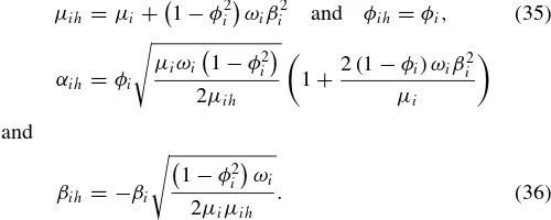
the GARCH option-pricing literature, it is standard to compute the volatility process using the GARCH volatility recursion, since the factors are observable. Factors in the SVS models, however, are latent, and we need to filter them to price op-tions. To remain consistent and facilitate comparison with the GARCH alternative, we develop a simple GARCH recursion that approximates the volatility dynamics in the SVS model by matching the mean, variance, persistence, and covariance with the returns of each volatility component. The dynamics of each volatility component is then approximated using Heston and Nandi’s (2000) GARCH recursion (Equation (3)), where the GARCH coefficients are expressed in terms of the associated SVS factor coefficients, as follows:
µih=µi+
1−φi2ωiβi2 and φih=φi, (35)
αih=φi
µiωi
1−φi2
2µih
1+2 (1−φi)ωiβ
2
i
µi
and
βih= −βi
1−φ2
i
ωi
2µiµih
. (36)
Our matching procedure can be viewed as a second-order GARCH approximation of the SVS dynamics, intuitively ana-logue to the approximation of the log characteristic function used by Bates (2006) when filtering affine latent processes.
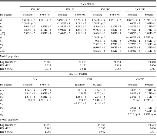
The top panel of Table 3reports the results of the option-based estimation for SVS models, and the bottom panel reports
the results of the GARCH alternative. All parameters are significantly estimated at the 1% level. Compared to historical parameters, the risk-neutral dynamics are more negatively skewed and the variance components are more persistent. These two findings are very common in the option-pricing literature. Higher negative skewness of the risk-neutral dynamics are reflected in higher negative values ofβi andηi estimates for
SVS models, and a larger negative value ofβih estimates for
GARCH models. For example, the estimated values ofβ1andη1 for the SVS1FU model are, respectively,−2450 and−0.2325 for the risk-neutral dynamics inTable 3, compared to−500 and
−0.00364, respectively, for the historical dynamics in Panel A ofTable 1. The persistence of the variance for the SVS1FU model is 0.9920 for the risk-neutral dynamics in Table 3 and 0.9824 for the historical dynamics in Panel A ofTable 1. The risk-neutral variance is more persistent than the physical variance. Also, note that, for the SVS2FU model, both volatility components are now very persistent under the risk-neutral dy-namics, with half-lives of 30 days for the short-run component and 385 days for the long-run component, compared to 3 days and 81 days, respectively, under the historical dynamics.
The last three rows of each panel inTable 3 show the log-likelihood, the IVRMSE metric of the models, and their ratios relative to HN. The IVRMSE for the restricted one-factor SVS model, SVS1FC, outperforms its one-factor GARCH competi-tors, HN and CHJ. The IVRMSE for the SVS1FC model is 3.56%, compared with 3.89% and 3.78% for HN and CHJ, corresponding to an improvement of 9.38% and 6.35%, re-spectively. Moving to the unrestricted one-factor SVS model, SVS1FU, considerably reduces the pricing error and yields an impressive improvement of 23.26% and 19.85% over HN and CHJ, respectively. This result illustrates the superiority of our conditional skewness modeling approach over existing affine GARCH, since CHJ has the same number of parameters as the SVS1FU model and more than the SVS1FC model. This re-sult also highlights the clear benefit of allowing more negative skewness in the risk-neutral conditional distribution of returns.
Table 3. Estimation results on S&P500 index options: SVS and GARCH models
SVS models
SVS1FC SVS1FU SVS2FC SVS2FU
Parameters Estimate Std error Estimate Std error Estimate Std error Estimate Std error
β1 −2.468E + 3 1.28E + 2 −2.450E + 3 8.02E+ 1 −1.046E + 4 1.15E+ 3 −1.847E + 4 2.80E+ 3 η1 0.000E + 0 –2.325E – 1 1.08E – 2 0.000E + 0 1.083E – 2 3.92E – 2 µ1 3.968E – 5 1.55E – 6 8.534E – 5 1.58E – 6 5.566E – 6 6.22E – 7 3.421E – 6 5.13E – 7 φ1 9.879E – 1 2.13E – 4 9.920E – 1 1.59E – 4 9.763E – 1 5.83E – 4 9.770E – 1 7.75E – 4
√ω
1 2.315E – 5 8.98E – 7 2.684E – 5 4.96E – 7 3.616E – 6 3.88E – 7 2.097E – 6 3.08E – 7
β2 0.000E + 0 −4.025E – 1 7.51E+ 1
η2 −1.975E – 1 5.88E – 3 −2.018E – 1 5.82E – 3
µ2 2.592E – 5 7.71E – 6 5.275E – 5 3.39E – 6
φ2 9.989E – 1 1.60E – 4 9.982E – 1 1.35E – 4
√ω
2 6.672E – 5 4.42E – 6 5.275E – 5 1.49E – 6
Model properties
Log-likelihood 20,100 21,080 21,851 21,880
IVRMSE 3.557 3.156 2.981 2.970
Ratio to HN 0.914 0.811 0.766 0.763
GARCH models
HN CHJ CJOW
Parameters Estimate Std error Estimate Std error Estimate Std error
µ1h 1.24E – 4 6.55E – 7 1.178E – 4 9.04E – 7 8.01E – 5 3.34E – 6
φ1h 9.85E – 1 8.97E – 5 0.9857 1.27E – 4 9.66E – 1 7.22E – 4
α1h 1.81E – 6 5.85E – 9 1.68E – 6 2.04E – 8 2.44E – 6 1.39E – 7
β1h 208.61 4.62E + 0 238.50 5.84E + 0 291.60 1.60E+ 1
η1h −2.17E – 3 8.45E – 5
φ2h 9.97E – 1 1.49E – 4
α2h 2.19E – 6 5.67E – 8
β2h 2.22E + 1 2.13E+ 0
Model properties
Log-likelihood 19,158 19,277 21,623
IVRMSE 3.890 3.783 3.000
Ratio to HN 1.000 0.972 0.771
We estimate the four SVS and the three GARCH models using option data for the period January 1, 1996, to December 31, 2004. Standard errors are computed using the outer product of the gradient.
Not surprisingly, the two-factor GARCH model (i.e., CJOW), with a RMSE of 3.00%, fits the option data better than both the one-factor GARCH and SVS models. In fact, as pointed out by Christoffersen et al. (2008) and Christoffersen et al. (2009), a second volatility factor is needed to fit appropriately the term structure of risk-neutral conditional moments. Our re-stricted two-factor SVS model, SVS2FC, has a comparable fit to CJOW, with a RMSE of 2.98%. The performance of the unconstrained two-factor SVS model is almost similar to the constrained version, reflecting the fact that bothη1 andβ2are not significantly estimated at the conventional 5% level. Option pricing thus seems to favor a risk-neutral distribution of stock prices that features a Gaussian as well as a negatively skewed shock; that is, a discrete-time counterpart to a continuous-time jump-diffusion model.
We further compare the performance of our SVS model specifications to variants of the SVJ model discussed in Section 3.3. For this second set of comparisons, we fit the option data using a well-known approach in the SV option-pricing
literature, an iterative two-step procedure, proposed, studied, and used by Bates (2000), Huang and Wu (2004), Christoffersen et al. (2009), and, more recently, by Andersen et al. (2012). The method consists of estimating both parameters and unobservable latent factors in two steps. In Step 1, for a given set of structural parameters, and a given timet, we minimize the pricing errors to get estimates of unobservable latent factors. In Step 2, given the set of latent factors estimated from Step 1, we solve one aggregate sum of squared pricing errors optimization problem to get a new estimation of the model parameters. The procedure iterates between Steps 1 and 2 until no further significant decreases in the overall objective in Step 2 are obtained.
The top panel ofTable 4reports the results of the option-based estimation for SVS models, and the bottom panel reports the results of the SVJ alternative, using the iterative two-step pro-cedure. All critical parameters are significantly estimated at the 1% level. SVS estimation results based on the iterative two-step procedure are comparable to those based on the approximate GARCH-like filtering method exploited earlier. With a RMSE
Table 4. Estimation results on S&P500 index options: SVS and SVJ models
SVS models
SVS1FC SVS1FU SVS2FC SVS2FU
Parameters Estimate Std error Estimate Std error Estimate Std error Estimate Std error
β1 −1.345E + 3 8.60E + 0 −1.994E + 3 2.20E+ 1 −1.293E + 3 1.63E+ 1 −1.994E + 3 3.83E + 1 η1 0.000E + 0 0.00E + 0 −8.468E – 1 2.12E – 2 0.000E + 0 −4.582E – 1 2.93E – 2 µ1 8.778E – 5 1.90E – 6 7.571E – 5 1.09E – 6 9.705E – 5 5.35E – 6 2.161E – 6 6.24E – 6 φ1 9.966E – 1 9.09E – 5 9.954E – 1 8.17E – 5 9.970E – 1 1.56E – 4 9.980E – 1 1.29E – 4
√ω
1 1.072E – 4 2.58E – 6 5.008E – 5 9.68E – 7 1.178E – 4 6.63E – 6 1.429E – 5 2.06E – 5
β2 0.000E + 0 −1.994E + 3 5.04E + 2
η2 −2.596E + 0 2.08E – 1 −9.768E + 0 1.02E + 0
µ2 1.886E – 7 2.41E – 8 1.602E – 4 2.09E – 5
φ2 9.958E – 1 2.83E – 3 9.686E – 1 2.60E – 3
√ω
2 1.125E – 4 7.17E – 5 1.217E – 5 3.56E – 6
Model properties
Log-likelihood 28,062 28,744 28,246 29,068
IVRMSE 1.717 1.551 1.617 1.512
Ratio to SV 0.979 0.884 0.922 0.862
Affine stochastic volatility/Jump models
SV SVJ0 SVJ1 SVJ
Parameters Estimate Std error Estimate Std error Estimate Std error Estimate Std error
αc 8.397E−7 9.66E−9 7.943E−7 9.11E−9 7.656 E−7 8.18E−9 6.684E−7 1.14E−8
βc 4.338E−3 6.50E−5 5.140E−3 7.66E−5 6.610E−3 1.06E−4 6.037E−3 1.06E−4
σc 1.296E−3 8.10E−6 1.260E−3 8.20E−6 1.237E−3 8.77E−6 1.156E−3 1.07E−5
ρc −8.698E−1 4.61E−3 −1.000E + 0 6.97E−3 −6.558E−1 5.75E−3 −6.753E−1 6.76E−3
λ0c 1.883E−5 2.28E−4 4.770E−16 9.66E−15
λ1c 4.506E−1 2.49E−5 4.415E−1 4.97E−2
¯
γc 9.655E−1 3.12E−1 −3.406E + 0 4.37E−1 −6.410E + 0 1.56E + 0
δc 2.684E−1 9.10E−2 2.626E−2 4.75E−2 3.019E−1 1.45E−2
Model properties
Log-likelihood 27,876 28,012 28,595 28,639
IVRMSE 1.754 1.697 1.532 1.521
Ratio to SV 1.000 0.968 0.873 0.867
We estimate the four SVS and four SVJ models using option data for the period January 1, 1996, to December 31, 2004. Standard errors are computed using the outer product of the gradient.
of 1.52%, the full SVJ specification with eight parameters just slightly outperforms the full one-factor SVS specification with five parameters and an RMSE of 1.55%. The full two-factor SVS model with 10 parameters has a RMSE of 1.51%, a fit that is comparable to the full SVJ specification. However, both the SVS1FU and the SVS2FU models achieve a higher likelihood compared to the SVJ models. We can then simply argue that SVS and SVJ models have a comparable fit on option prices, and we recall from Section4.2results that SVS models outperform the SVJ model in fitting the historical distribution of returns.
Overall, the results of model estimation based on option data confirm the main conclusions from the GMM estimation based on returns in Section4.2. Both conditional skewness in returns and a second volatility factor are necessary to reproduce the observed stylized facts, and disentangling the dynamics of con-ditional volatility from the dynamics of concon-ditional skewness offers substantial improvement in fitting the distribution of as-set prices.
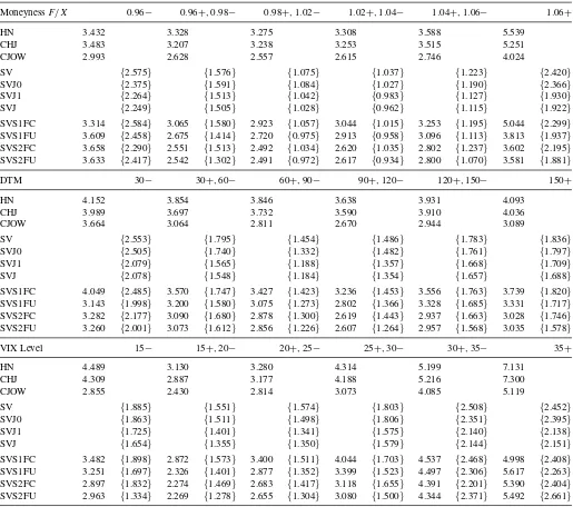
InTable 5, we dissect the overall IVRMSE results reported in Tables3and4, by sorting the data by moneyness, maturity, and VIX levels, using the bins fromTable 2. The top panel of Table 5reports the IVRMSE for the various SVS, GARCH, and SVJ models by moneyness. Comparing SVS versus GARCH, we see that the two-factor models, with the lowest overall IVRMSE in Table 3, also have the lowest IVRMSE in each of the six moneyness categories. The benefits offered by the two-factor models are therefore not restricted to any particular subset of strike prices. Note that all models tend to perform worst for deep out-of-the-money put options (F /X >1.06), also corresponding to the highest average implied volatility, as shown by the top panel ofTable 2. For example, HN, CHJ, and the SVS1FC model fit deep OTM options with IVRMSEs of 5.54%, 5.25%, and 5.04%, respectively. With a fit of 4.02%, CJOW is outperformed by the SVS1FU, the SVS2FC, and the SVS2FU models, which have fits of 3.81%, 3.60%, and 3.58%, respectively.
Table 5. IVRMSE option error by moneyness, maturity, and VIX level
MoneynessF /X 0.96− 0.96+,0.98− 0.98+,1.02− 1.02+,1.04− 1.04+,1.06− 1.06+
HN 3.432 3.328 3.275 3.308 3.588 5.539
CHJ 3.483 3.207 3.238 3.253 3.515 5.251
CJOW 2.993 2.628 2.557 2.615 2.746 4.024
SV {2.575} {1.576} {1.075} {1.037} {1.223} {2.420}
SVJ0 {2.375} {1.591} {1.084} {1.027} {1.190} {2.366}
SVJ1 {2.264} {1.513} {1.042} {0.983} {1.127} {1.930}
SVJ {2.249} {1.505} {1.028} {0.962} {1.115} {1.922}
SVS1FC 3.314 {2.584} 3.065 {1.580} 2.923 {1.057} 3.044 {1.015} 3.253 {1.195} 5.044 {2.299}
SVS1FU 3.609 {2.458} 2.675 {1.414} 2.720 {0.975} 2.913 {0.958} 3.096 {1.113} 3.813 {1.937}
SVS2FC 3.658 {2.290} 2.551 {1.513} 2.492 {1.034} 2.620 {1.035} 2.802 {1.237} 3.602 {2.195}
SVS2FU 3.633 {2.417} 2.542 {1.302} 2.491 {0.972} 2.617 {0.934} 2.800 {1.070} 3.581 {1.881}
DTM 30− 30+,60− 60+,90− 90+,120− 120+,150− 150+
HN 4.152 3.854 3.846 3.638 3.931 4.093
CHJ 3.989 3.697 3.732 3.590 3.910 4.036
CJOW 3.664 3.064 2.811 2.670 2.944 3.089
SV {2.553} {1.795} {1.454} {1.486} {1.783} {1.836}
SVJ0 {2.505} {1.740} {1.332} {1.482} {1.761} {1.797}
SVJ1 {2.079} {1.565} {1.188} {1.357} {1.668} {1.709}
SVJ {2.078} {1.548} {1.184} {1.354} {1.657} {1.688}
SVS1FC 4.049 {2.485} 3.570 {1.747} 3.427 {1.423} 3.236 {1.453} 3.556 {1.763} 3.739 {1.820}
SVS1FU 3.143 {1.998} 3.200 {1.580} 3.075 {1.273} 2.802 {1.366} 3.328 {1.685} 3.331 {1.717}
SVS2FC 3.282 {2.177} 3.090 {1.680} 2.878 {1.300} 2.619 {1.443} 2.937 {1.663} 3.028 {1.746}
SVS2FU 3.260 {2.001} 3.073 {1.612} 2.856 {1.226} 2.607 {1.264} 2.957 {1.568} 3.035 {1.578}
VIX Level 15− 15+,20− 20+,25− 25+,30− 30+,35− 35+
HN 4.489 3.130 3.280 4.314 5.199 7.131
CHJ 4.309 2.887 3.177 4.188 5.216 7.300
CJOW 2.855 2.430 2.814 3.073 4.085 5.119
SV {1.885} {1.551} {1.574} {1.803} {2.508} {2.452}
SVJ0 {1.863} {1.511} {1.498} {1.806} {2.351} {2.395}
SVJ1 {1.725} {1.401} {1.341} {1.575} {2.140} {2.138}
SVJ {1.654} {1.355} {1.350} {1.579} {2.144} {2.151}
SVS1FC 3.482 {1.898} 2.872 {1.573} 3.400 {1.511} 4.044 {1.703} 4.537 {2.468} 4.998 {2.408}
SVS1FU 3.251 {1.697} 2.326 {1.401} 2.877 {1.352} 3.399 {1.523} 4.497 {2.306} 5.617 {2.263}
SVS2FC 2.897 {1.832} 2.274 {1.469} 2.683 {1.417} 3.118 {1.655} 4.391 {2.201} 5.390 {2.404}
SVS2FU 2.963 {1.334} 2.269 {1.278} 2.655 {1.304} 3.080 {1.500} 4.344 {2.371} 5.492 {2.661}
We use Wednesday closing out-of-the-money (OTM) call and put option data from OptionMetrics from January 1, 1996, through December 31, 2004.Fdenotes the implied futures price of the S&P500 index,Xdenotes the strike price, and DTM denotes the number of calendar days to maturity. We report IVRMSE from the models estimated inTable 3by moneyness, maturity, and VIX level. The entries not in curly brackets represent IVRMSE for the estimation based on GARCH updating of the volatility factors, while the entries in curly brackets are based on the iterative two-step procedure. All IVRMSE values are in annualized percentage points.
For deep-in-the-money options (F /X <0.96), CJOW has the best fit, an IVRMSE of 2.99%, compared to more than 3.31% for any other concurrent model. For all other moneyness categories, CJOW and the two-factor SVS models have comparable fits, the difference in their IVRMSEs being less than 0.10%. The perfor-mance of the SVS1FU model is very consistent across strikes as well, the best among the one-factor models. Thus, contrary to the historical dynamics of returns, contemporaneous asymmetry appears to be important in characterizing the risk-neutral dynam-ics, and the low IVRMSE of the SVS1FU model compared to the SVS1FC model across all categories demonstrates the impact of the significant and negative estimate ofη1reported inTable 3.
The middle panel ofTable 5reports the IVRMSE across ma-turity categories. Again we see that all two-factor models have a comparable fit across all maturity categories, but the short-est maturity (DTM<30) where the two-factor SVS models
perform better compared to CJOW. The SVS1FU model still outperforms any other one-factor competitor along the matu-rity dimension. While all models have relatively more difficulty fitting the shortest and the longest maturity compared to inter-mediate maturity options, our results show the superiority of the SVS over the GARCH regarding the shortest maturity op-tions. With an IVRMSE of 3.14% for this category, the SVS1FU model provides the best SVS fit, while the best GARCH fit of 3.66% is due to CJOW.
The bottom panel ofTable 5reports the IVRMSE across VIX levels. The two-factor models provide the best fit across the six VIX categories, and the SVS1FU model remains the best one-factor fit along this dimension. All models have difficulty fitting options when the level of market volatility is high (V I X≥
35%), since, for all models, the IVRMSE is the highest for these VIX levels.