www.elsevier.nl / locate / econbase
Tax limits and the qualifications of new teachers
a b ,*
David N. Figlio , Kim S. Rueben a
Department of Economics, University of Florida, Florida FL, USA b
Public Policy Institute of California, 500 Washington street, San Francisco CA 94111, USA Received 1 February 1999; received in revised form 1 August 1999; accepted 1 January 2000
Abstract
This paper examines the impact of local tax limits on new teacher quality. Using data from the National Center for Education Statistics we find that tax limits systematically reduce the average quality of education majors, as well as new public school teachers in states that have passed these limits. The average relative test scores of education majors in tax limit states declined by ten percent as compared to the relative test scores of education majors in states that did not pass limits. This relationship is strengthened if we control for school finance equalization reforms or examine tax limits passed in two different periods.
2001 Elsevier Science B.V. All rights reserved.
JEL classification: H73; I21
1. Introduction
The existing empirical evidence suggests that teacher quality is extremely important in determining student outcomes (see, e.g., Rivkin et al., 1998). While there have been several prominent proposals in recent years to increase teacher salaries to encourage higher-quality entrants into the teaching force, in policy the last few years have been marked more by voter initiatives and legislation more likely to substantially cut school revenues, and potentially, teacher salaries. In 1996, for instance, there were nine tax limitation initiatives on the ballots of eight
*Corresponding author. Tel.:11-415-291-4414; fax:11-415-291-4428.
E-mail address: [email protected] (K.S. Rueben).
1
states, of which seven passed. The number of such initiatives has been increasing since 1990, and is rapidly approaching the level witnessed during the ‘tax revolt’ of the late 1970s and early 1980s.
The existing evidence concerning the effects of tax revolt-era limits on student outcomes (Figlio, 1997; Downes and Figlio, 1997) suggests that tax limits have led to substantial declines in student test performance, at least in mathematics. This may come as a surprise to those familiar with the ‘education production function’ literature (see, e.g., Hanushek’s (1986) survey article and subsequent updates) that suggests that school spending has at most a small influence on student outcomes. Understanding why tax limits may lead to decreased student outcomes when money per se may not matter much is of great interest, but to date, the only potential intermediate links explored in the literature – money, student-teacher ratios, and student-teacher salaries – seem unlikely to explain much of this discrepancy, given that these factors are also generally found to have little or no effect on outcomes. An alternative link may involve teacher quality: several recent authors, including the paper by Rivkin et al. (1998) mentioned above, have found a strong link between teacher quality and student outcomes. Tax limits might affect the qualifications of new teachers if relatively high-quality potential teachers expect salaries or working conditions to decline after the limit’s passage, and disproportionately choose not to enter teaching in an affected state. (Of course, high-quality existing teachers may also differentially select out of teaching.) However, almost nothing is known about the effects of large-scale (expected) reductions in school spending on the quality of the teaching force, and even the political debate surrounding the tax limitations has been silent on this issue.
This paper is the first to explore the effects of widespread and large-scale changes in school finance on the qualifications of the teaching force. For this project, we focus on the effects of tax limitations, the largest-scale and most visible (as well as the most currently relevant) changes in school finance policies. It is important to study the effect of tax limits themselves, rather than the relationship between teacher salaries and teacher qualities, to gauge the effects of this recent ‘tax revolt,’ for several reasons. Tax limits are likely to affect potential teachers in multiple dimensions, and the mechanism through which tax limits work is almost surely not exclusively through teacher salaries. Prior empirical evidence suggests that tax limits affect both teacher salaries as well as student-teacher ratios (Figlio, 1997), suggesting that tax limits may lead to longer queues for teaching jobs at stated wage rates. In addition, the larger class sizes and lower spending on
1
non-salary instructional expenses associated with tax limits, and possible associ-ated changes in school composition, imply more complicassoci-ated effects on career choices. Hence, we study the effects of tax limits directly.
We exploit unique, detailed individual-level data on three nationally-representa-tive cohorts of potential teachers, spanning twenty years from the mid-1970s to the mid-1990s, and relate tax limitation imposition to the probability that a potential teacher of any given qualification level will select into a career in education. We take advantage of the fact that with three cohorts of data and two distinct rounds of tax limitations since the mid-1970s, we can distinguish the effects of tax
2
limitations on the quality of new teachers in a state from ‘naturally-occurring’ trends in a state’s new teacher quality level. Therefore, we can make projections about the longer-run consequences of the recently-passed and currently-proposed set of fiscal constraints. Our research suggests that tax limitations significantly reduce the quality level of entrants into a state’s teaching force.
2. Tax limits and the test scores of education majors
We are interested in gauging whether the passage of tax and expenditure limits has systematically affected the quality of individuals entering the teaching force. To do so, we must gather data on the relative quality of new teachers across states, before and after the passage of tax and expenditure limits. The approach we take is as follows: we first use two nationally representative longitudinal data sets, the National Longitudinal Survey of the High School Class of 1972 (NLS-72) and the High School and Beyond (HSB) survey (sophomore cohort) to get, in essence, two cohorts of potential teachers, one that graduated from high school and selected college majors well before the tax revolt of the late 1970s, and the other that graduated high school after the tax revolt had passed (as they would be high school graduates in 1982). In each of these data sets, all high school seniors took a series of academic examinations in mathematics and verbal ability. Since we know the discipline into which each college-attending sample member selected, we can determine whether there are systematic differences in academic ability between those who select into education and those who do not in each cohort. We can then investigate whether the passage of tax limits has systematically affected this difference, and in which direction.
To address this question, we must have a measure of academic ability that can be compared across time. Fortunately, both NLS-72 and HSB tested every student in each respective cohort in mathematics and verbal ability. The two rounds of
2
tests are measured in different units, but can be adjusted so that they are directly
3
comparable.
Almost without exception, teachers in the United States have at least a bachelor’s degree. When we compare ability levels of people selecting into education to others, we must choose a comparison group with a comparable level of education. Therefore, we limit our sample to individuals who have graduated from college by the last round of each sample (1986 for the NLS-72 cohort; 1992 for the HSB cohort). We have also experimented with restricting this ‘completion by’ date for the NLS-72 cohort to 1978, for fear that we might have a few individuals in the NLS-72 cohort who attended college and chose their majors
after the tax revolt had begun. It turns out that this sampling modification does not
change our estimated parameters of interest in any substantive way. In all, we have 1,450 observations with complete data in the NLS-72 cohort and 2933 observa-tions with complete data in the HSB cohort, for a total of 4,383 observaobserva-tions. Of these, 477 individuals, or 11%, selected into an education major.
Since we are interested in estimating the effect of the passage of tax and expenditure limits on a college student’s decision of whether to major in education, we must first address the question: whose tax limit is relevant? Does the student respond to a tax limit in his or her home state, for instance, or a tax limit in the state in which he or she is attending college? Evidence from the NLS-72 suggests that the second option is probably more likely: in the cases in which a student attends a college out of state, college students are more likely to remain in the state where they attended college than return to the state in which they
4
graduated from high school. Therefore, the results that we report in this paper count as the relevant tax limit any policy changes that take place in the state in
which the individual attends college. As a sensitivity test, we have also estimated
our models in which the relevant policy changes are those that take place in the
3
We perform this adjustment as follows: We assume that any given score on the ACT test is time-invariant (that is, a ‘23’ on the ACT in 1972 means the same thing as a ‘23’ on the ACT in 1982). Since a sizeable subset of each cohort took the ACT exam, we can use the ACT as a benchmark to determine a score matching between the NLS-72 and HSB. For the students in each cohort who took the ACT, we regress the student’s ACT score on the relevant test’s composite (verbal plus math) ability score. Details on these regressions are available on request. We use these regression results to construct an ‘ACT-equivalent’ score for every student in both cohorts. Using this algorithm, we convert each NLS-72 student’s test score into HSB units. (The ACT is simply used to scale the test scores to make them directly comparable; our sample consists of every student in the data sets, not just ACT exam-takers.) These corrections are almost exactly the same if we use SAT scores instead to calibrate test scores over time.
4
5
state where the student attended high school; it turns out that this modification barely changes the parameter estimates of interest.
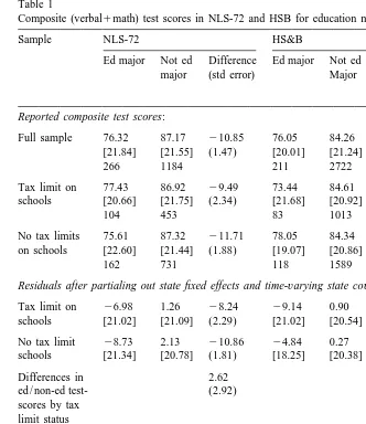
We initially present some basic descriptive analysis. The top panel of Table 1 compares college graduates with education majors to college graduates majoring in other fields in both cohorts of students. The first row of the table reports mean HSB-equivalent test scores, by cohort and major. Each cell also presents the standard deviation (in square brackets) and the number of observations within that category for illustrative purposes. We observe that in both cohorts, education majors average considerably lower test scores than do non-education majors. In the NLS-72 (students who graduated from high school in 1972), education majors averaged almost eleven points or one-half of a standard deviation lower on the
6
ACT-normed test than did non-education-major college graduates. This gap had shrunk to a still sizeable and statistically significant 8 points (or .4 standard deviations) by the HSB cohort (students who graduated from high school in 1982). We then compare education majors to non-education majors in states that passed tax limits vs. those that did not pass tax limits. The results of these comparisons are reported in the next two rows of Table 1. In the NLS-72, our pre-tax revolt cohort, we find that education majors in states that would eventually pass tax limits averaged 9.5 points lower test scores than did non-education majors, while education majors in states that never passed tax limits averaged nearly 12 points
7
lower (or one-half of a standard deviation) than did non-education majors. By the HSB, after tax revolt-era limits were passed, these relative levels had been reversed. Education majors in tax limit states averaged 11 points lower on the achievement tests than did non-education majors (that is, the gap widened even as nonmajor achievement fell slightly in limit states), while the gap between education majors and non-education majors in no-limit states fell to only 6 points or to one-third of a standard deviation of average test scores. Therefore, the qualitative evidence suggests that while states that never passed tax limits saw a
5
While the NLS-72 identifies the school district attended by students, the restricted-access version of the HSB does not even identify the state where the student went to high school. However, the identities of colleges attended are reported in HSB. Therefore, we say that the high school’s state (in the HSB cohort) is the state where the largest number of students from that school eventually attended college. This, of course, is not an issue at all for our reported specifications, as we know the state in which each student attended college.
6
This percentage figure, and subsequent ones, are constructed by dividing the reported difference (in this case,210.85) by the basis for the comparison (in this case, 87.17).
7
Table 1
a Composite (verbal1math) test scores in NLS-72 and HSB for education majors and non-majors
Sample NLS-72 HS&B Difference
between Ed major Not ed Difference Ed major Not ed Difference
teachers major (std error) Major
and non-teachers
Reported composite test scores:
Full sample 76.32 87.17 210.85 76.05 84.26 28.21 [21.84] [21.55] (1.47) [20.01] [21.24] (1.51)
266 1184 211 2722
Tax limit on 77.43 86.92 29.49 73.44 84.61 211.17 schools [20.66] [21.75] (2.34) [21.68] [20.92] (2.39)
104 453 83 1013
No tax limits 75.61 87.32 211.71 78.05 84.34 26.29 on schools [22.60] [21.44] (1.88) [19.07] [20.86] (1.98)
162 731 118 1589
Residuals after partialing out state fixed effects and time-varying state covariates:
Tax limit on 26.98 1.26 28.24 29.14 0.90 210.04 schools [21.02] [21.09] (2.29) [21.02] [20.54] (2.35) No tax limit 28.73 2.13 210.86 24.84 0.27 25.11 schools [21.34] [20.78] (1.81) [18.25] [20.38] (1.93)
Differences in 2.62 24.93
ed / non-ed test- (2.92) (3.03)
scores by tax limit status
Difference in difference in difference 27.55 25.58 (4.09) (3.48)
Excluding California for analysis 28.34 25.73
(4.39) (3.96) Controlling for the presence of legislative and 27.92 25.63 court-mandated school finance reforms (4.12) (4.19)
Controlling for the presence of pro- 29.85 26.47
spending and anti-spending reforms, as (3.99) (3.61) designated by Hoxby (1996)
a
decrease in the gap between education majors and non-education majors over the decade encompassing the tax revolt, this gap in tax limit states actually increased by 17%. Moreover, the average absolute test score of education majors in tax limit states fell over this decade as compared to a modest increase in absolute test scores of education majors in non tax revolt states.
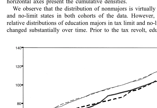
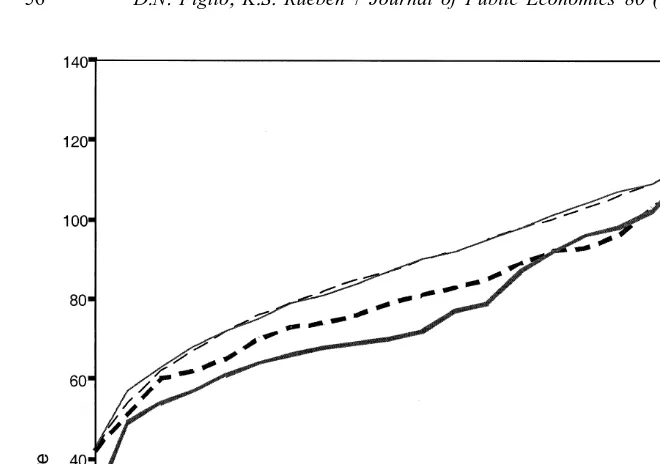
From the above information, it is clear that the test scores, which we are using as our proxy of average ability level, of education majors vs. nonmajors in tax limit states and no-limit states has changed over time. It may also be interesting to gauge the apparent effect of tax limits on the overall distribution of academic ability of education majors and nonmajors. Have all quantiles of the distribution shifted in the same direction (and with the same magnitude) as the mean? To address this question, we present in Figs. 1 and 2 the cumulative density functions (cdfs) of the test levels of education majors and nonmajors in tax limit and no-limit states. Fig. 1 presents these cdfs for the NLS-72 sample, before the tax revolt, while Fig. 2 presents these cdfs for the HSB sample, after the tax revolt. Note that the vertical axes of these figures present the distribution of test scores while the horizontal axes present the cumulative densities.
We observe that the distribution of nonmajors is virtually identical in tax limit and no-limit states in both cohorts of the data. However, we observe that the relative distributions of education majors in tax limit and no-limit states apparently changed substantially over time. Prior to the tax revolt, education majors in tax
Fig. 2. Distribution of education majors and non-majors following tax revolt (HSB subsample).
limit and no-limit states had comparable test distributions, except that the bottom quartile of education majors in tax limit states had qualitatively higher scores than did the bottom quartile of education majors in no-limit states. After the tax revolt, however, these two distributions spread more appreciably apart. While the top quartiles of education majors in tax limit and no-limit states maintained compar-able achievement levels, at all other points of the distribution relative education major achievement is substantially lower in tax limit states, relative to no-limit states. The most noticeable differences take place in the bottom third of the distribution, where test scores of education majors and nonmajors converged to a large degree in no-limit states but not in tax limit states.
The above comparisons may be plagued by omitted variables bias. For instance, suppose that the sampled education majors from tax limit states came from systematically different backgrounds in one round of data than in the other round (say, different states end up better represented in one sample than in the other). Alternatively, perhaps there are other factors, such as cyclical changes, that are correlated with both states that passed tax limits and average ability levels of individuals selecting into teaching. As a first attempt to deal with this possibility, we compare the relative mean test scores of education majors and nonmajors in tax limit and no-limit states before vs. after the tax revolt, after controlling for
the state’s population that is school-aged, and per capita personal income in the
8,9
state.
The results of these comparisons are presented in the bottom panel of Table 1. We observe that, as before, we find opposite trends in tax-limit and no limit states.
While the gap in (residual) ability decreased by half (from 210.86 to 25.11) in
states that did not pass a tax and expenditure limit over this time period, the gap
increased (from 28.24 to 210.04) in the states that passed tax limits during the relevant period. Therefore, after controlling for state and year effects and two time-varying state-specific factors, we still find that tax limits are associated with decreases in teacher ability, relative to the changes in teacher ability that occurred in no-limit states.
We can use these differences in mean residuals to estimate a treatment effect of tax limits on relative education major quality. To do so, we adopt a differences-in-differences-in-differences estimation strategy, similar to that used by Gruber and Madrian (1994), except that we further control for time-invariant state-specific effects. Essentially, we wish to determine whether the change over time in the ability gap between education majors and non-education majors differs sys-tematically depending on whether the student’s state passed a tax limit during the intermediate period. Our results are difference-in-difference-in-difference results because they represent the difference between tax limit states and no-limit states in the difference between the mid-1970s and the mid-1980s in the difference between education major and non-major test scores.
The cell in Table 1 marked ‘difference in difference in difference’ presents the
estimated parameterd in the equation
test score5QX1ayear (Y )1blimit (L )1jstate (S )1g edmajor (E )
1zY*L1hY*E1lE*L1d*E*L*Y1e
where individual and time subscripts are assumed but omitted and Y5h0 if
NLS-72 (pre tax revolt) and 1 if HSB (post revolt)j and X is a vector of
time-varying state-specific factors. (We include the parameter b in the equation
above for illustration, though in practice it is subsumed into the state effect
(b 1j).) We can interpretdas the difference between tax limit states and no-limit
8
We also tested our specification by including a number of other state specific variables including population, total state income, percent of the population over 65 and under 5 and a measure of the state’s liberalness based on the state’s US Senators’ scores on selected votes as determined by Americans for Democratic Action. The results did not change significantly when these variables were included and the extra variables had no predictive power once state fixed effects were added. Nor do the results change if only these other covariates are included.
9
states in the change from the NLS-72 cohort to the HSB cohort in the test-score gap between education majors and non-education majors, holding constant
observable characteristics. A negative value of d would indicate that, all else
equal, the ability gap between education majors and non-education majors has widened since the tax revolt in tax limit states, relative to no-limit states. While our data samples are representative of the nation as a whole, they are not necessarily representative of individual states at any given time, as the data are drawn from clustered, multi-stage sampling frameworks. Moreover, our policies in question vary only at the state level in any given year. Therefore, we correct all standard errors for within-state, within-time error correlation and heteroskedasticity using the approach described by Moulton (1990); this standard error correction also
ensures that we are estimating our models as if we have 48 states 3 2 time
periods596 effective observations. Recall that an effective observation is the
difference between education majors and non-majors.
We observe a negative and statistically significant relationship between tax limits and the relative ability level of education majors relative to non-education majors. This 7.55 point change in the relative ability level of education majors translates into a 10% decrease in ability level or about four-tenths of a standard deviation change in the high-school test scores of potential teachers when evaluated at the mean value. This result is statistically significant at traditional
10
levels.
Might our results be driven by California? California’s Proposition 13 is the most famous of the tax revolt era limits, and California accounts for 22% of the observations in our sample in tax limit states. To check, we estimate our difference-in-difference-in-difference model excluding California from the sample. We find that, if anything, the results just get stronger: the estimated treatment
effect of tax limits is now 28.34, with a robust standard error of 4.39.
Our results may also be confounded by the fact that many states enacted school finance reforms over the same period. Therefore, the final two cells in Table 1
present the estimated parameter d in an equation in which we also include a
10
separate set of school finance reform variables in the model. To address this, we first control for the implementation of either court-mandated or
legislatively-11
mandated school finance reforms, as identified by Downes and Shah (1995). We
find qualitatively similar though slightly larger results.
Next, we take to heart Hoxby’s (1996) concern that not all school finance reforms are created equal, and that some ‘no-reform’ states saw substantially larger changes in the state’s school finance formula than did some ‘reform’ states. Here, we replace the school finance reform variables described above with two sets of reform variables and interactions, one set each for the states that implemented pro-spending and anti-spending school finance reforms, as defined by Hoxby
12
(1996). We again find estimated tax limit treatment effects that, if anything, are
slightly larger than those found when not controlling for the presence of school
finance reforms: the estimated treatment effect is 29.85, with a standard error of
3.99. While the Hoxby classification and the Downes and Shah classification of school finance reforms are just two of a number of approaches to characterizing finance reforms, the fact that our results hold up to controlling for various characterizations of school finance reforms suggests that the treatment of school finance reforms is unlikely to substantively influence our estimated tax limit effects.
This portion of our analysis, therefore, leads to several distinct conclusions. First, we present significant evidence that tax revolt-era tax and expenditure limits have led to an increase in the ability gap between education majors and non-education majors in the affected states. This effect is not only statistically significant, but is substantial in magnitude as well. Finally, we find that controlling for whether the state also passed school finance reforms is unimportant in gauging the degree to which the tax limits affected education major quality. It is interesting to note that the difference-in-difference-in-difference coefficients on the school finance reform variables are generally not statistically significant, nor are they typically sizeable in magnitude. Therefore, while we find substantial evidence that
11
On this basis, states that passed school finance reforms during the relevant time period were Arkansas, California, Connecticut, Kansas, Kentucky, New Jersey, Utah, Washington, West Virginia, Wyoming and Arizona, Florida, Georgia, Idaho, Illinois, Iowa, Maine, Maryland, Massachusetts, Minnesota, Missouri, New Hampshire, New Mexico, Ohio, Oklahoma, Rhode Island, South Carolina, South Dakota, Tennessee, Vermont, Virginia and Wisconsin. The first set of states passed court mandated reforms while the second set of states passed state legislated school finance reforms.
12
tax limits led to diminished education major quality, we generally cannot differentiate from zero the parallel effect of school finance reforms.
2.1. Additional sensitivity testing
It is still possible that our results are being driven by some omitted variable associated with both the passage of tax revolt-era limits and changes in the ability level of individuals selecting into being an education major in those states. This concern would be mitigated if we were to find similar types of results looking at an entirely different round of tax limits. Fortunately, from a research perspective, there has been another recent round of tax limits, with Arizona, Colorado, Illinois, Iowa and Oregon each passing a new tax limit between 1989 and 1992. Therefore, we can perform a similar type of analysis looking at the estimated effect of this new round of tax caps.
To do so, we repeat the analysis presented in Table 1, but this time with two different data sets – the High School and Beyond sample described above (to reflect conditions before the new round of tax caps) and the National Education Longitudinal Survey (NELS), a national longitudinal survey of eighth-graders conducted first in 1988, so it is representative of the high school class of 1992. Our NELS data are not as ideal for this analysis as are the HSB and NLS-72 data, because we only know students’ college major choices up to the fall of their junior year, and it’s possible that some students might fail to complete college or might change majors between their junior and senior years. We have reason to believe, however, that this is not likely to be the case. Using data from the HSB, we find that among declared education majors in the fall of their junior year, fewer than 4% end up switching to a different major, and fewer than 3% of students who eventually became an education major had not done so by their junior year. Moreover, there is no significant difference in HSB test scores of students who switch late into education vs. those who declare an education major early, and there is no significant difference in test scores between students who choose a non-education major late vs. those that make such a choice early. Therefore, a snapshot of the college major choices of sample members as college juniors in the NELS is likely to fairly accurately reflect the eventual distribution of education majors and nonmajors.
Our NELS sample is somewhat larger than either of our prior rounds: we have 4671 observations in the NELS sample, and of these, 507 are education majors. Almost 10% of HSB observations are in states with new tax limits, and 7.6% of NELS observations are in states with new tax limits. Means and distributions of education major and nonmajor adjusted test-scores, by tax limit status (both rounds), for all three rounds of data, are reported in Appendix A.
Table 2
Difference-in-difference results for a different round of tax limits: estimated effects of 1990s-era tax a
limits
Difference between Difference between education majors and education majors and nonmajors in HSB nonmajors in NELS
New tax limit states 22.19 21.90
(1.21) (2.65)
States without new tax 27.87 22.56
limits (1.32) (0.98)
Difference in difference 5.68 0.65
(1.71) (2.58)
Difference in difference in 25.03
difference (3.13)
Controlling for the presence 25.45
of school finance reforms (3.32)
a
Standard errors of differences, reported beneath point estimates in parentheses, are corrected for within state-time correlation in the errors. The results above control for state and year fixed effects and time varying state characteristics.
correct standard errors for within-state-time correlation in the errors. As with the first round of tax limits, education majors in states that would eventually pass 1990s-era tax limits began the sample in a better relative position, ability-wise, than did education majors in the control group of states. However, over the ensuing decade, education majors in no-limit states closed two-thirds of the test-score gap with nonmajors, while the gap remained virtually unchanged in the tax limit states. The difference between (new) tax limit states and no-limit states in the before-after difference in the education major-nonmajor ability gap is therefore negative, and statistically significant, at least at the 10% level. The magnitude of
the estimated effect of the new tax limits, 25.45, is similar if a little smaller, to
that found regarding the earlier round of tax limits. Controlling for the presence of school finance reforms, as before, slightly strengthens the results. (Here, we focus only on court-ordered and legislative school finance reforms, as Hoxby’s study only classifies school finance reforms up to 1990.)
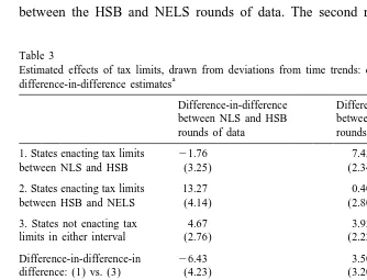
data to estimate the effects of tax limits on relative education major quality as a deviation from a state-specific trend. We operationalize this by classifying the states into three groups: (1) states with tax revolt-era tax limits, (2) states with 1990s-era tax limits, and (3) states with tax limits in neither period. We then calculate differences between time periods in the differences-in-differences-in-differences between the groups of states. The resulting difference-in-difference-in-difference-in-difference represents the estimated deviation from trend associated with a tax limit introduced in a particular time period. In the remainder of the paper, we are referring to this estimation technique when we discuss ‘deviation from trend.’
Table 3 presents the results of this exercise. The first cell in the first row presents the difference between NLS-72 and HSB in the difference between average education major and nonmajor test scores in states passing tax revolt-era tax limits. The second cell in the first row makes the same comparison, but between the HSB and NELS rounds of data. The second row reports the same
Table 3
Estimated effects of tax limits, drawn from deviations from time trends: difference-in-difference-in-a
difference-in-difference estimates
Difference-in-difference Difference-in-difference between NLS and HSB between HSB and NELS rounds of data rounds of data
1. States enacting tax limits 21.76 7.43
between NLS and HSB (3.25) (2.34)
2. States enacting tax limits 13.27 0.40
between HSB and NELS (4.14) (2.80)
3. States not enacting tax 4.67 3.93
limits in either interval (2.76) (2.22)
Difference-in-difference-in 26.43 3.50
difference: (1) vs. (3) (4.23) (3.20)
Difference-in-difference-in- 29.93 difference-in-difference: (5.30) Estimated effect of first
round of tax limits
Difference-in-difference-in- 8.60 23.52
difference: (2) vs. (3) (4.82) (3.47)
Difference-in-difference-in- 212.12
difference-in-difference: (5.94)
Estimated effect of second round of tax limits
a
analysis for the states passing tax limits in the later round, while the third row presents the same results for states not passing tax limits in either period.
The fourth row of the table presents difference-in-difference-in-difference results when comparing tax revolt states to states never enacting tax limits. We observe that, relative to never-passing-limit states, tax revolt states saw relative decreases in relative education major ability levels between the NLS and HSB rounds of data, and small relative gains in relative education major ability levels in the period with no change in tax limit activity. This deviation from trend
(presented in the fifth row), therefore, is estimated to be 29.93 and significant at
conventional levels.
The sixth row of the table presents difference-in-difference-in-difference results when comparing new tax limit states to states never enacting tax limits. We observe that, relative to never-passing-limit states, 1990s-era tax limit states saw differential increases in relative education major ability levels between the NLS and HSB rounds of data, and differential decreases in relative education major ability levels in the latter period when the change in tax limits occurred. The implied effect of 1990s-era tax limits, when expressed as a deviation from trend, is
estimated to be 212.12 and is also significant at conventional levels. Therefore,
when we use data from three rounds of data, and calculate tax limit effects as deviations from trends, our estimated effects of tax limits only become stronger. We observe that the average quality of education majors fell in ‘first round’ tax limit states relative to no-limit states between the mid-1970s and mid-1980s, but then rebounded in part between the mid-1980s and the mid-1990s. There are a number of possible explanations for this finding. One could be that states that enacted tax limits were on a faster growth path (in terms of teacher quality) than were no-limit states, and that this growth was interrupted by the imposition of a tax limitation. If this is the case, then the observed rebounding of ‘first round’ limit states would be entirely expected. There is reason to believe that this may be the case: note that states that enacted ‘second round’ tax limits saw significantly greater relative growth in education major quality between the mid-1970s and mid-1980s than did no-limit states, in a period in which schools in both set of states were not fiscally constrained. The evidence presented in Figlio (1997) that ‘first round’ tax limit states tended to more strongly support education prior to the tax revolt than did no-limit states also supports this notion. Furthermore, data from the SASS suggests that teacher salaries grew faster, and student-teacher ratios fell faster, in ‘first round’ limit states than in no-limit states between 1987 and 1993, also supportive of the hypothesis that our estimated results are causal. This partial rebound of teacher quality (as well as school resources), if symptomatic of a lessening of the constraints imposed by tax limits, could also help explain the passage of multiple limits over time in certain states.
that high-quality potential teachers will enter education. One candidate explanation is that tax limits are correlated with a temporary increase in political conservatism in a state, that is also associated with a decline in the desire of high-quality potential teachers to select into education. We have strong reason to believe that this is not the case. As mentioned in footnote 6, our results are unchanged when we include as controls measures of liberalness / conservativeness like the average Americans for Democratic Action scores of the state’s Senators or members of Congress. A simple exploration of the data suggests that the change in the liberalness of representatives of ‘first round’ tax limit states and no-limit states is nearly identical between the early 1970s and early 1980s (a change of 6 points more liberal for tax limit states and 5 points more liberal for no-limit states), and only between the early 1980s and early 1990s did the two sets of states diverge. However, in that period, the trend was that no-limit states tended to trend more liberally than ‘first round’ tax limit states. Therefore, it is highly unlikely that differential conservative sentiment could have driven these results.
3. Changes in attributes of new teachers
The results presented in the preceding discussion suggest that tax limits have had substantial negative effects on the average relative test-scores of education majors. But this is only an imperfect approximation of the effects of tax limits on
teacher quality. While the vast majority of them do, not all education majors
eventually become teachers. In addition, not all public school teachers were education majors in college. Therefore, it is always possible that the decrease in the overall ability level of education majors as an apparent consequence of tax limits is not an accurate representation of what actually happened to the average ability level of teachers in general.
the average ability level of private school teachers in a state is time-invariant, we cannot use the available data to directly estimate the effect of tax limits on public school teacher ability levels.
Despite these shortcomings, there is still utility in estimating our Table 1 model in which we explore the differences between people employed as teachers to those not employed as teachers, instead of making education major-nonmajor com-parison. We report the estimated tax limit effects in this model in the final column of Table 1. We observe that the estimated effect of tax limits on teacher quality is
25.58 with a standard error of 3.48, statistically significant at the 11% level.
Omitting California, or controlling for different representations of school finance reforms, yields results of the same magnitude, and the results just strengthen in statistical significance if we estimate a one-observation-per-state-year sample, as we did with the education major sample. Moreover, these results are almost certainly biased toward zero, because we cannot distinguish between teachers in the public and private sectors, and because we cannot distinguish between teachers who teach in the same state as their college degree and those who changed states. In sum, the results are very similar whether we estimate the model using education majors or using all teachers as a proxy for public school teachers.
That the results are similar across specifications is not surprising, given the high degree of overlap between education majors and eventual teachers. In the NLS-72 data, 82% of education majors eventually became teachers, and more than two-thirds of teachers, public or private, were education majors in college. In addition, there is no statistically significant difference between the test scores of education majors who eventually taught and those who did not teach, and if anything, education majors who eventually did not teach tended to score slightly
higher than education majors who eventually taught. In the HSB data, the fraction
of education majors who eventually taught is somewhat lower (about 70%), as is the fraction of public or private school teachers who were education majors (about 61%), but there remains no perceptible difference between education majors who eventually taught and education majors who never taught. Therefore, there is no evidence to suggest that our results are merely picking up the weakest college students, who entered an education major because of a perception that it is the ‘easiest,’ but never become teachers.
3.1. Evidence from the schools and staffing surveys
colleges the teachers in the SASS attended, we can approximate relative teacher ability with an indicator of whether the college attended is selective (as identified
13
by Peterson’s Guides.) College selectivity of teachers has been shown (e.g., by
Loury and Garman, 1996) to be strongly related to their underlying test scores, and has also been shown (e.g., by Ehrenberg and Brewer, 1994, and Ferguson, 1991) to be strongly independently correlated with the academic achievement of students they teach.
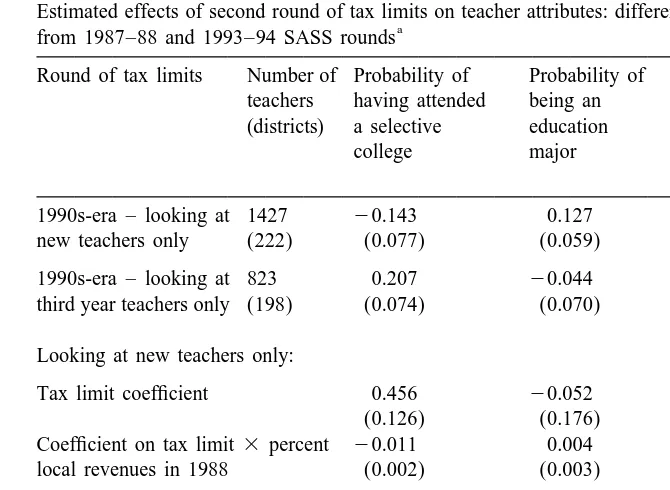
Two rounds of the SASS, 1987–88 and 1993–94, identify the colleges attended by the sampled teachers. This set of samples also spans the ‘second round’ of tax limits described in Tables 2 and 3. The SASS has the advantage of having thousands of new teachers, so measurement error is less likely to be an issue here than in the preceding analysis. The first row of Table 4 presents the estimated effect of tax limit imposition on the probability of attending a selective college or being an education major by brand-new teachers, that is, teachers who began working at their school within the year preceding the 1993–94 SASS sample. As before, we control for cohort effects in tax limit and no limit states, the percentage of the state population that is school-aged during the appropriate cohort, and state per-capita income during the relevant period. Given the size of our sample, in the specification reported we control for time-invariant school district specific effects. Also, as before, we correct our standard errors for the presence of within-state-cohort correlation in the errors using the procedure described by Moulton (1990). Our sample consists of teachers in school districts with at least three new teachers in the SASS in each cohort. Our results do not change substantially if we omit the school district-specific effect. For ease of interpretation, we report the results of linear-probability models, but the results are quite similar if we were to estimate conditional logit models instead.
We estimate that tax limits are associated with about 14 percentage points’ lower probability of a new teacher having graduated from a selective college. (About 63% of teachers in our sample graduated from a selective college.) This effect is statistically significant at conventional levels, and suggests that tax limits led to reductions in the quality of teachers entering the teaching force.
It may, however, still be the case that, even if teachers are more likely to graduate from a less prestigious college, they might have come from a higher point in the college’s skill distribution, so that the true quality of teachers did not fall with tax limits. We can indirectly test this proposition in several ways. First, we estimate a model in which the dependent variable is the probability that a new teacher was an education major in college; this is intended to capture the fact that
13
Table 4
Estimated effects of second round of tax limits on teacher attributes: difference-in-difference estimates a
from 1987–88 and 1993–94 SASS rounds
Round of tax limits Number of Probability of Probability of Probability of teachers having attended being an being an education (districts) a selective education major, conditional on
college major attending a selective college
1990s-era – looking at 1427 20.143 0.127 0.105 new teachers only (222) (0.077) (0.059) (0.077) 1990s-era – looking at 823 0.207 20.044 0.042 third year teachers only (198) (0.074) (0.070) (0.139) Looking at new teachers only:
Tax limit coefficient 0.456 20.052 20.200
(0.126) (0.176) (0.159)
Coefficient on tax limit3percent 20.011 0.004 0.006 local revenues in 1988 (0.002) (0.003) (0.003) Estimated effect for 25th percentile 20.071 0.150 0.097 of percent local in 1988 (0.071) (0.054) (0.071) Estimated effect for 50th percentile 20.174 0.190 0.156 of percent local in 1988 (0.068) (0.054) (0.067) Estimated effect for 75th percentile 20.426 0.287 0.298 of percent local in 1988 (0.080) (0.090) (0.092)
a
Standard errors of differences, reported beneath point estimates in parentheses, are corrected for within state-time correlation in the errors. The results above control for school district and year fixed effects and time varying state characteristics.
education majors consistently tend to rank at the bottom of their college’s distribution, on average, in test scores. The result presented in the second column of Table 4 suggests that tax limits increased the probability that a new teacher will be an education major by 13 percentage points, a result also statistically significant at conventional levels. Next, we estimate the probability that a new teacher will be an education major, conditional on having graduated from a selective institution. We observe that tax limits increase the probability of this occurring by 11 percentage points, although this result is only significant at the 17% level. Nonetheless, the results suggest that tax limits result in fewer new teachers who graduated from selective institutions and more new teachers who were education majors in college, and likely more education majors among the smaller set of teachers who attended selective colleges.
As an additional sensitivity check, we can compare recent but slightly older
want to compare teachers with exactly the same degree of seniority in their school district in the two rounds of data – but with no difference in the state’s tax limit
status of the states at the time of their hiring because the tax limit had not yet been
enacted in the second round. Here, we compare teachers in the same school districts with three years of seniority in 1987–88 and in 1993–94, in states that passed 1990s-era tax limits vs. those that did not. We find, consistently, that if anything, new teacher quality might have been improving in 1990s-era tax limit states prior to the tax limits’ imposition relative to no-limit states, but that in the years immediately following the new limits’ imposition this trend reversed. Therefore, we can more forcefully rule out that some time-varying unobserved feature correlated with tax limit imposition is driving our SASS results.
3.2. Within-state heterogeneity in tax limit effects
Using the SASS data, we can exploit more variation than we can using the longitudinal data presented in section 2 of this paper. Specifically, we can exploit the fact that tax limits tended to affect different school districts in the same state differentially. Therefore, in the third and fourth rows of Table 4, we present the results of a model in which we interact our tax limitation dummy variable with the fraction of school district revenues coming from local sources in 1988, before any
14
of the new wave of tax limits took place. Here, we are again using our sample of
new teachers. We observe that the estimated effects of tax limits on new teacher quality in the SASS data tend to increase in magnitude with the fraction of pre-tax limit revenues raised locally. The interaction terms are statistically significant at conventional levels when explaining the probability of a new teacher having attended a selective college, or the probability of a new teacher being an education major, conditional on having attended a selective college.
To aid in the interpretation of these results, in the fifth through seventh rows of Table 4 we present the implied effects of tax limits when the fraction of revenues raised locally is low (the 25th percentile among school districts in new tax limit states, a share of 46%), average (the median fraction raised locally, a share of 55%), and high (the 75th percentile, a share of 77%.) We estimate, for example, that the probability that a new teacher will have graduated from a selective college decreases by 7 percentage points (not significant) when prelimit local revenue share is low, but by 42 percentage points (and statistically significant) when pre-limit local revenue share is high. The estimated probability that a new teacher will have been an education major increases by 15 percentage points when pre-limit local revenue share is low, as compared to 29 percentage points when
14
pre-limit local revenue share is high (both are statistically distinct from zero, but are distinct from each other at only the 16% level). Conditional on having
graduated from a selective college, the estimated probability that a new teacher will have been an education major increases by 10 percentage points when pre-limit local revenue share is low, but by 30 percentage points when pre-limit local revenue share is high. The fact that the estimated effects of tax limits on new teacher quality vary with the pre-limit fraction of revenues raised locally lends additional evidence that our estimated relationships are causal.
4. Conclusion
This paper provides the first evidence of the relationship between tax limits and new teacher quality. Our research provides consistent evidence that tax limits systematically reduce the quality on average of education majors, as well as new public school teachers. Since prior authors have demonstrated a strong link between teacher quality and student outcomes, our result provides an explanation for why tax limits are negatively related to student test performance, as shown by Figlio (1997) and Downes and Figlio (1997). If, on average, high-quality potential teachers respond to tax limits by choosing not to teach in the public schools, states that have recently enacted (or are considering enacting) tax limits may expect to experience a resulting reduction in the average level of new teacher quality.
Acknowledgements
Appendix A. Means and standard deviations of high school and beyond-equivalent 12th grade test scores: By college major and state tax limit status
NLS (High school class HSB (High school class NELS (High school class
of 1972) of 1982 of 1992)
Group of Education Nonmajors Education Nonmajors Education Nonmajors
states majors majors majors
Tax revolt 77.43 86.92 73.44 84.61 73.95 77.36
era [20.66] [21.75] [21.68] [20.92] [20.39] [22.81] tax limits
1990s-era 73.83 89.82 79.81 82.96 78.87 80.97
tax [25.88] [20.50] [16.33] [19.99] [15.60] [21.81] limits
Never 75.85 86.90 77.75 84.59 78.26 81.29
enacted [22.22] [21.58] [19.55] [21.01] [20.63] [21.47] tax limits
References
Downes, T., Figlio, D.,1997. School finance reforms, tax limits, and student performance: do reforms level up or dumb down? Paper Presented at the 1998 Meetings of the Econometric Society. Downes, T., Shah, M., 1995. The effect of school finance reform on the level and growth of per pupil
expenditures. Tufts University Working Paper No. 95–4. Tufts University, Medford MA. Ehrenberg, R., Brewer, D., 1994. Do school and teacher characteristics matter? Evidence from high
school and beyond. Economics of Education Review. 13, 1–17.
Ferguson, R., 1991. Paying for public education: new evidence on how and why money matters. Harvard Journal on Legislation 28 (Summer), 465–498.
Figlio, D., 1997. Did the ‘Tax Revolt’ reduce school performance? Journal of Public Economics 65 (September), 245–269.
Figlio, D., 1998. Short-run effects of a 1990s-era property tax limit: Panel evidence on Oregon’s measure 5. National Tax Journal 51 (March), 55–70.
Gruber, J., Madrian, B., 1994. Health insurance and job mobility: The effects of public policy on job-lock. Industrial and Labor Relations Review 48 (October), 86–102.
Hanushek, E., 1986. The economics of schooling: production and efficiency in public schools. Journal of Economic Literature 49 (3), 1141–1177.
Hoxby, C., 1996. All school finance equalizations are not created equal: marginal tax rates matter. National Bureau of Economic Research, Working Paper 6323, Massachusetts.
Loury, L., Garman, D., 1996. College selectivity and earnings. Journal of Labor Economics. Moulton, B., 1990. An illustration of a pitfall in estimating the effects of aggregate variables on micro
units. Review of Economics and Statistics 72 (May), 334–338.
Rivkin, S, Hanushek, E, Kain, J., 1998. Teachers, schools, and academic achievement. National Bureau of Economic Research Working Paper 6691, Massachusetts.