Lessons From The Weakest Link
Kate Antonovics
Peter Arcidiacono
Randall Walsh
A B S T R A C T
We use data from the television game show, The Weakest Link,to determine whether contestants discriminate on the basis of race and gender and, if so, which theory of discrimination best explains their behavior. Our results sug-gest no evidence of discriminatory voting patterns by males against females or by whites against blacks. In contrast, we find that in the early rounds of the game women appear to discriminate against men. We test three theories for the voting behavior of women: preference-based discrimination, statisti-cal discrimination, and strategic discrimination. We find only preference-based discrimination to be consistent with the observed voting patterns.
I. Introduction
The earnings of both women and blacks have consistently lagged behind those of white men. Empirically determining whether these differences arise because of discrimination is extremely difficult, and distinguishing between the vari-ous theories of discrimination is harder still. As a result, researchers have begun to look outside of labor markets to develop a better understanding of whether and why individuals discriminate. This paper builds on the emerging experimental literature on discrimination and explores the use of a high-stakes game environment to reveal pat-terns of discrimination. To this end, we use data from the television game show The
Kate Antonovics is an assistant professor of economics at the University of California, San Diego. Peter Arcidiacono is an assistant professor of economics at Duke University. Randall Walsh is an assistant pro-fessor of economics at the University of Colorado at Boulder. The authors thank Vince Crawford, Nora Gordon, Roger Gordon, Tom Nechyba, Joel Watson, and seminar participants at the University of Colorado, Johns Hopkins University, and the University of Pennsylvania for their helpful comments and advice concerning this paper. The authors also thank Patrick Dickinson and Pamela Maine for research assistance. The data used in this article can be obtained beginning May 2006 through April 2009 from Peter Arcidiacono, Department of Economics, Duke University, Durham, NC 27708-0097, email: psar-cidi@econ.duke.edu.
[Submitted June 2004; accepted March 2005]
ISSN 022-166X E-ISSN 1548-8004 © 2005 by the Board of Regents of the University of Wisconsin System
Weakest Linkto determine whether contestants discriminate on the basis of race and gender, and, if so, which theory of discrimination best explains their behavior.
A number of existing papers analyze contestant behavior on television game shows in order to draw inferences about behavior in more policy-relevant settings.1The bene-fit of this type of analysis is twofold. First, in many situations, the strategic environment of game shows generates data that can be used to answer questions that cannot be eas-ily addressed with data from more traditional settings. This is particularly relevant in the context of labor market discrimination where economists have had only limited success at distinguishing between the various theories of discrimination using standard data. Second, the stakes are much larger on game shows than in laboratory experiments and these stakes may influence both the extent and nature of discrimination. For example, Ball and Eckel (2003) find that favoritism toward members of “high status” groups in ultimatum games is sensitive to the dollar value of the prize being split.
The principal feature of The Weakest Linkthat enables us to study discrimination is the fact that players have multiple opportunities to cast votes against their fellow con-testants in order to remove them from the game. As a result, we are able to examine whether race and gender play a role in determining voting patters. In addition, we are aided by the fact that the data from the show provide excellent controls for individual ability. This is important since one of the principal difficulties in establishing the pres-ence of discrimination is that it is almost impossible to determine whether unequal outcomes arise because of discrimination or because of unobservable race and gender differences in productivity. However, in The Weakest Link we observe the same explicit measure of individual ability—the percentage of questions answered cor-rectly—that is observed by the contestants. Our ability to observe a large fraction of the information that the contestants have about one another limits the extent of the omitted variables bias problem that plagues discrimination research. Further, even if there remain important unobserved characteristics, the structure of the game allows us to control for these omitted factors by using information on the voting patterns of the other contestants. In particular, if we are trying to examine the factors that determine whether Player A votes against Player B, we can control for the proportion of other contestants who vote against B. In this way, we can account for other factors that are not directly included in our data but that are relevant to the players’ voting decisions. In addition, because data are collected from two slightly different versions of the show, a daily show and a weekly show, the veracity of our results can be tested against two independent samples.
The structure of the game also allows us to examine why contestants discriminate. In particular, we are able to distinguish preference-based discrimination (in which dis-crimination arises because people simply do not like members of certain groups) from statistical discrimination (in which discrimination arises because people use group identity as a proxy for unobserved ability). In a strategic environment such as The Weakest Link, we also need to consider a third type of discrimination: what we term “strategic discrimination.” The notion here is that in a strategic setting race and gen-der may serve as focal points for collusive behavior (see, for example, Holm 2000).
Antonovics, Arcidiacono, and Walsh 919
A major contribution of this paper is to highlight various methods of distinguishing between these three theories of racial discrimination.
To look for evidence of discriminatory behavior, we evaluate the voting decisions of individual players using a series of conditional logit models. A major advantage of the conditional logit model relative to analysis of the total votes cast against a partic-ular group is that it allows us to consider interactions between the characteristics of the individuals doing the voting and the characteristics of those receiving the votes. Thus, for example, one can examine whether men are more likely to vote against women andwhether women are more likely to vote against men. The results reveal no evidence of discrimination against either women or blacks. However, we consis-tently find that women are substantially more likely to vote against men in the early rounds of the game, even after controlling for a broad set of performance measures. That is, based on these findings, it appears that women discriminate against men (and in favor of women) in their voting decisions. We are able to show that neither statis-tical discrimination nor strategic discrimination explains this pattern. Instead, the evi-dence seems broadly consistent with women simply preferring to play the game with other women.
At first glance, it may seem surprising that we find no evidence of discrimination against women or blacks. However, the data reveal no significant race or gender dif-ferences in contestants’ ability to answer questions correctly. As a result, even if sta-tistical discrimination is a feature of the labor market, we are able to rule it out as a possible source of discrimination in our data.2Thus, given that we find no evidence of preference-based discrimination or strategic discrimination against women or blacks, our results point toward statistical discrimination as a possible explanation for the discriminatory patterns found in studies of the labor market.
Interestingly, the notion that women have discriminatory preferences in favor of other women is reflected in a number of recent studies. For example, Dillingham, Ferber, and Hamermesh (1994) examine male and female voting behavior in the selection of officers for a professional association. Confirming our results, they find that men do not discriminate on the basis of gender while women discriminate in favor of female candidates.
II. Previous Work on Racial Discrimination
A. Evidence From the Labor Market
It is not surprising that there exists an enormous literature on racial and gender dis-crimination in the labor market. Here we divide these studies into two groups: those that test for evidence of discrimination and those that attempt to distinguish between different theories of discrimination.
One approach to testing for evidence of discrimination is to run wage regressions that control for individual-level characteristics (see, for example, Altonji and Blank 1999 for a full discussion). However, it is well-known that the estimated race and gender wage
differentials from these regressions should not necessarily be interpreted as evidence of discrimination. The primary problem is that unobservable individual-level characteris-tics that are correlated with race and gender may lead to estimated race and gender wage differentials even in the absence of discrimination. A second problem is endogeneity bias. Many individual-level characteristics that we would like to include as controls may be influenced by discrimination. For example, because blacks tend to have lower levels of experience than whites, it would seem natural to include experience in the wage regressions. However, if blacks have lower levels of experience because of past dis-crimination, then including experience will lead the coefficient on race to understate the true extent of discrimination. Thus, while wage regressions often provide interesting descriptions of the data, they do not provide solid evidence of discrimination.
A second strand of the literature uses audit studies to look for evidence of discrim-ination (Cross, Kenny, and Zimmerman 1990; Turner, Fix, and Struyk 1991; Neumark 1996). The majority of these studies find substantial evidence of discrimination against women and blacks in both the labor and housing markets. However, as Heckman and Siegelman (1992) and Heckman (1998) point out, these studies may fail to overcome the omitted variables bias that plagues standard regression techniques. In particular, the implicit assumption of audit studies is that the auditors are identical apart from their race and gender. However, the researcher who selects the auditors may not know or may not be able to observe all of the characteristics that are relevant to employers. Thus, if there is any relationship between race and gender and these unobserved components, then the differences in outcomes across these groups may not truly represent discrimination.
Two studies that circumvent this problem are Goldin and Rouse (2000) and Bertrand and Mullanaithan (2004). Goldin and Rouse examine whether the adoption of “screens” that hide the identity of auditioning musicians from judges has been respon-sible for the increase in the proportion of females hired at orchestras. Overall their evi-dence is consistent with discrimination against female musicians, and indicates that the use of the screen has been responsible for a large fraction of the increase in the num-ber of women hired. Bertrand and Mullanaithan (2004) conduct a field experiment in which they send out a series of resumes to employers in the Boston and Chicago areas that are essentially identical apart from the name at the top of the page.3They find that the response rates on resumes with white-sounding names are 50 percent higher than those with African American names. While both of these provocative studies find evi-dence of discrimination, they do not fully reveal whythe discrimination occurs.
Within the field of economics, the two leading theories of discrimination are pref-erence-based discrimination and statistical discrimination. In models of preference-based discrimination, employers act as if there is some cost associated with hiring workers from a particular group, and, in equilibrium, workers from these groups are paid lower wages than workers from other groups (Becker 1957). In contrast, in mod-els of statistical discrimination firms cannot perfectly observe worker productivity, and base their assessment of worker productivity on prior beliefs about the produc-tivity of workers in different groups. Thus, discrimination can arise either because of group differences in average productivity or in the quality of information that firms
Antonovics, Arcidiacono, and Walsh 921
have about workers. (See, for example, Phelps 1972; Arrow 1973; Aigner and Cain 1977; Lundberg and Startz 1983; Coate and Loury 1993.)
A handful of studies explicitly test for evidence of preference-based discrimination. Three of these, Ashenfelter and Hannan (1986), Hellerstein, Neumark, and Troske (2002), and Kahn and Sherer (1988), find evidence consistent with preference-based discrimination. A smaller number of studies test for evidence of statistical discrimi-nation. For example, both Oettinger (1996) and Altonji and Pierret (2001) build mod-els of statistical discrimination in which employers slowly learn about worker quality. Unfortunately, their models generate conflicting predictions about what differences in black-white age-earnings profiles imply about statistical discrimination.4
B. Evidence From Experiments
Complementing the empirical work on labor markets are a number of papers by both psychologists and economists that look for evidence of discrimination in laboratory settings. A common finding is that individuals display “in-group bias” in the sense that they favor members of their own group (for example, Turner 1978; Turner and Brown 1978; Vaughn, Tajfel, and Williams 1981). The evidence also suggests that group status plays a role in determining the outcome of bargaining games (Ball et al. 2001). A number of papers also look for evidence of statistical discrimination in lab-oratory settings (for example, Anderson and Haupert 1999; Davis 1987; Fryer, Goeree, and Holt 2005). These papers consistently show that statistical discrimination tends to arise in the presence of incomplete information. Generally, the groups defined in these settings are artificial. (For example, the groups might be “green” and “yel-low.”) One exception is Fershtman and Gneezy (2001) who analyze discrimination among Ashkenazic and Eastern Jews. They find discrimination against Eastern Jews in “trust” games by both Ashkenazic and Eastern Jews. Conducting a series of exper-iments, Fershtman and Gneezy argue that this result is due to incorrect expectations regarding the “trustworthiness” of Eastern Jews.
Simultaneous to our paper, Levitt (2004) also examines discrimination in The Weakest Link.5Our approaches are very different. Levitt focuses on aggregate dis-crimination (total votes cast against a particular group) rather than whether discrimi-nation against a given group depends on the demographics of those doing the voting. For instance, we are interested in determining whether women vote against men and whether men vote against women, effects that are not observable and may cancel each other out under Levitt’s approach.6Levitt’s results also differ from our own because of differences in our interpretation of the strategic incentives in the game. In particu-lar, Levitt’s method relies on two assumptions. First, in Levitt’s paper the extent of
4. Oettinger interprets the earnings gap between blacks and whites increasing over the life-cycle as evidence for statistical discrimination while Altonji and Pierret interpret the same feature as evidence against statisti-cal discrimination.
5. Indeed, in late December of 2002, we both found out the other was close to completing their project. The result was two January 2003 working papers.
taste-based discrimination must be the same across all rounds of the game. However, because the implicit cost of taste-based discrimination rises as the game progresses (because one’s probability of winning the game is higher in later rounds), discrimina-tory outcomes due to taste discrimination should diminish over time. Second, Levitt assumes that voting incentives switch as the game progresses, so that contestants first want to vote off weak players and later want to vote off strong players. Given the structure of the game, it is not clear that the voting incentives will truly reverse. We find that although the incentives to vote off the weakest player diminish as the game progresses, at no point is the strongest player ever more likely to be voted off than the weakest player. An advantage of Levitt’s work is that he has a larger sample of daily shows and analyzes discrimination against the elderly and Hispanics.
III. Data and Rules of the Game
We focus on the version of The Weakest Link produced by NBC Enterprises and broadcast in the United States. Our data come from our own video recordings of more than 100 episodes.
There are two versions of The Weakest Linkan hour long weekly show and a half-hour long daily show, with both versions following the same general structure. After excluding celebrity episodes where the contestants play for charity, our data consist of 28 weekly shows and 75 daily shows.7Each show is divided into a series of timed rounds, with the number of rounds corresponding to the number of players: eight rounds in the weekly show and six rounds in the daily show. Within each round, play-ers are sequentially asked to answer general trivia questions where correct answplay-ers translate to an increase in the prize money. The first correct answer is worth $1,000 in the weekly show and $250 in the daily show. After a correct answer, a player can choose to “bank” the money for the team. If the player banks, the next correct answer is again worth $1,000 in the weekly show and $250 in the daily show. Should the player decide not to “bank,” the amount of money added to the pot following a cor-rect answer increases. However, failure to answer a question corcor-rectly leads to the loss of any unbanked money for that round. A successive chain of eight (six) correct answers with no intermittent “banks” leads to a $125,000 ($12,500) increasein the pot. Money banked from each round is accumulated into a team bank.
After each round, each player votes independently as to which player he would like to remove from the show, and the player who receives the most votes must leave the game. In the event of a tie, the “strongest link” chooses which player to remove from the subset of players who received the most votes. The strongest link is the player who answers the highest percentage of his or her questions correctly. Once the field of players is reduced to two (this occurs in Round 7 of the weekly show and Round 5 of the daily show), these two players first accumulate prize money in the same fashion as in the earlier rounds, after which the two players compete directly against each other with the winner taking all the money in the team bank.8
Antonovics, Arcidiacono, and Walsh 923
7. The data are incomplete for some rounds due to broadcast interruptions.
One drawback of our data is that the contestants on The Weakest Linkare unlikely to be representative of the U.S. population. Indeed, this problem plagues much of the experimental literature. We have investigated how contestants are selected to be on the The Weakest Link. The show draws contestants from a diverse set of groups. Besides variation in gender and race, contestants come from a broad range of ages, occupa-tions and educational backgrounds. As with most television game shows, the most significant criterion for selection is whether the contestant is telegenic. We have no a priori reason to believe this is correlated with discriminatory behavior.
IV. Why Discriminate on
The Weakest Link?
The Weakest Linkprovides a unique environment in which to distin-guish between various theories of discrimination. Playing the game well not only involves answering questions correctly, but also making astute inferences about the other players’ ability to play the game. Because we observe players’ decisions about who to vote off, we can determine whether race and gender are relevant factors in vot-ing decisions even after controllvot-ing for each player’s performance.
In addition, we examine why contestants discriminate. Complicating this analy-sis is the game’s evolving strategic environment. In the early stages of the game, when the contestants act cooperatively to build the pot of prize money, there is a clear incentive to vote off weak players. Indeed, in Round 1 of the daily show, the weakest player is voted off over 50 percent of the time, while the strongest player is voted off only 4 percent of the time. However, voting incentives may shift as the game progresses. As discussed above, in the final round, the two remaining players first build the pot of prize money cooperatively as they do in earlier rounds. Then they face one another in a head-to-head competition to determine the winner of the entire game. Thus, concern about the head-to-head competition creates an incentive to vote off strong contestants, particularly in later rounds. It is unclear, however, whether the incentive to vote off strong players will outweighthe incentive to vote off the weak players because even in the final round the players cooperatively build the prize money. Empirically, we find that even though the probability of voting off the weakest link diminishes as the game progresses, players are always more likely to vote off the weakest link than the strongest link. Nonetheless, due to the ambi-guity in voting incentives and the complications associated with updating beliefs and incorporating past voting behavior into current voting behavior, we base the majority of our analysis on the first round of the game where voting incentives are more clear-cut.
Antono
vics, Arcidiacono, and W
alsh
925
Type of Discrimination Empirical Prediction
1. Preference-Based Discrimination Contestants will be more likely to vote against members of other groups.* Discrimination will become less pronounced as the game progresses since the implicit cost of discrimination increases at the end of the game.
2. Statistical Discrimination
a. Real group differences in average ability. There will be group-level differences in the percentage of questions answered correctly.*
Contestants from all groups will be more likely to vote against members of a single group.*
b. Contestants have better information Contestants will be more likely to vote against members of their own group.* about the ability of members of their
own group.
c. Inaccurate prior beliefs about a group’s
average ability. There will be a weaker pattern of discrimination in shows in which contestants are drawn from the same occupation.*
3. Strategic Discrimination
a. Explicit collusion Votes of members of a particular group will be correlated even after controlling for the votes of nongroup members. This also tests for implicit collusion based on observable characteristics.*
b. Implicit collusion If a group successfully votes off a nongroup member in one round, then the group will be more likely to vote against a nongroup member in the subsequent round.
Figure 1
A. Statistical Discrimination
Contestants in this game may use race and gender as proxies for underlying ability. In this setting, discriminatory voting patterns can arise either because of real group differences in ability or because some contestants have better information about the ability level of one group relative to another. These two sources of statistical discrimination (differences in ability vs. differences in the quality of information) yield different predictions about voting patterns.
To see this, assume that there are two groups: Group A and Group B, and that con-testants from Group A play the game better than concon-testants from Group B. If the incentives are such that players wish to remove weak players, then contestants from bothgroups should be more likely to vote against members of Group B. Likewise, if the incentives are to vote off stronger players, then both groups should be more likely to vote against members of Group A. One simple method for examining whether this type of statistical discrimination accounts for observed voting patterns is to look for group-level differences in the percentage of questions answered correctly during the first round of the game. Further, if there are real group differences in average ability, then we would expect members of all groups to vote against members of a single group.
Now, suppose instead that contestants from Group A and Group B are equally skilled, but contestants are better able to evaluate the ability of contestants within their own group. For example, in the context of the show, women may be better able to assess whether or not another woman should be able to answer a given question cor-rectly. In this case, contestants will place a relatively high weight on average ability when assessing the ability of players from other groups. That is, players from Group A will perceive a contestant from Group B with a below-average performance in Round 1 to be of higherability than a contestant from Group A with that same per-formance. As a result, contestants will be morelikely to cast votes againstmembers of their own group. This occurs regardless of whether or not the incentives are to vote off strong or weak players since players have better information about who the weak-est and strongweak-est players are within their own group. Thus, information is harmful. The exact opposite occurs in hiring practices where workers from groups that emit noisy productivity signals are relatively unlikely to be hired.
prior beliefs as a source of discriminatory voting behavior. A formal derivation of our predictions regarding statistical discrimination is presented in the Appendix.
B. Strategic Discrimination
In a strategic setting such as The Weakest Link,collusion also may play a role in dis-criminatory outcomes and may be the mechanism through which contestants either statistically discriminate or exhibit discriminatory preferences. Statistical discrimina-tion can take this form when it is easier to form collusive agreements within one’s own group, and preference-based discrimination can take this form when contestants pre-fer own-group agreements to cross-group agreements. Two types of collusion are pos-sible here: explicit collusion (where particular contestants follow some agreed upon pattern of voting) and implicit collusion (where no agreements are discussed but indi-viduals play strategies that yield focal points).
Contestants meet one another prior to the game and presumably have opportunities to discuss (quite possibly collusive) strategies for playing the game. These collusive agree-ments may be more likely to occur among members of the same race or gender. If con-testants are explicitly colluding, they should not only be more likely to vote against nongroup members, but also should be more likely to vote against the samenongroup member. To test for explicit collusion, we examine whether the votes of the contestants are correlated with the votes of contestants from their own group. Because there may be unobservable characteristics that make particular individuals more likely to be voted off, in this analysis we also control for the votes cast by nongroup members.
If we find that votes are no more correlated within a group than outside the group, then we are also able to rule out many other forms of discrimination. Namely, if one group is discriminating based upon an unobservable individual level characteristic that is correlated with membership in another group, then this too will lead to corre-lation in within group voting.
Discriminatory outcomes also may result from implicit collusion where individu-als naturally play particular equilibria. For example, discriminating against members of Group B may be a best response for members of Group A given that the other members of Group A are playing a discriminatory equilibrium. These focal point equilibria should be reinforcing. Hence, if Group A succeeds in removing a member of Group B in Round 1, then this should make it more likely that they will vote against a member of Group B in Round 2. We can therefore test for implicit collusion by examining how who is voted off in one round affects voting behavior in the next round. Note that testing for implicit collusion based upon an unobservable feature cor-related with group membership is embedded in the test for explicit collusion. This is because, given this style of implicit collusion, within group votes will be correlated after controlling for the votes of others and the group membership.
C. Preference-Based Discrimination
In the prototypical model of preference-based discrimination, members of the major-ity group simply dislike working with members of the minormajor-ity group and act as if there is some nonmonetary cost associated with hiring them. As a result, in equilib-rium, workers from minority groups will earn lower wages than workers from
preferred groups. In The Weakest Link,contestants from one group may dislike playing the game with contestants from some other group. Thus, if we believe that members of Group A dislike members of Group B, we would expect that members of Group A would be consistently more likely to vote off members of Group B in every round. As the game progresses, however, the probability that any single player will win the game increases. As a result, the implicit cost of preference-based discrimination alsoincreases. For this rea-son alone, even if the contestants have discriminatory preferences, their propensity to dis-criminate will fade as the game progresses. Therefore, if preference-based discrimination exists, we would expect it to diminish with each round of the show.
V. Which Contestants Discriminate?
A. Descriptive Evidence
In order to understand the broad patterns in the data, we start by analyzing voting pat-terns by gender and race. Table 1 summarizes the voting behavior by round for both the daily and weekly shows. The table evaluates the voting behavior of three demo-graphic groups—men, women, and whites—to determine if members of these groups discriminate against players who are not group members. For example, do men dis-criminate against women in their voting patterns? The voting behavior of blacks is not considered due to the small number of episodes with two or more black contestants.
The task of discerning discrimination is complicated because even if both men and women vote randomly, men will cast more votes against women and women will cast more votes against men simply because a contestant will never vote against him or her self. To account for this problem, and the fact that the distribution of demographic types varies across episodes and rounds, we describe the voting behavior in terms of the mean “group bias statistic.” For individual ivoting in round r, the “group bias statistic” is given by:
(1) .
where 1iris an indicator variable that takes on a value of one if individual ivotes against
a contestant from his or her group in Round r. Giris the number of contestant i’s type in
Round rof his or her episode and Nris the total number of contestants in Round rof
contestant i’s episode. A mean value of one for the group bias statistic implies no dis-crimination, a value less than one implies discrimination against the other group and, and a value greater than one implies discrimination against one’s own group.
The descriptive evidence shows some surprising results. First, there is virtually no evidence of discrimination by whites against blacks; all of the values of our discrim-ination statistic are indistinguishable from one. Second, there is no discrimdiscrim-ination against women by men in the early rounds, though in Round 3 of both shows men are more likely to vote against women.9The most surprising result, however, is that in
Antono
vics, Arcidiacono, and W
alsh
929
Table 1
Own-Group Bias Statistic
Females Males Whites
Standard Standard Standard
Show/Round Sample Mean Deviation Sample Mean Deviation Sample Mean Deviation
Daily
1 222 0.739* 1.141 222 0.976 1.220 331 0.949 0.634
2 189 0.783* 1.212 186 1.336 0.336 235 0.982 0.703
3 150 0.910 1.177 123 0.756* 1.205 119 0.966 0.856
4 66 0.909 1.003 62 0.935 1.006 68 1.000 1.007
Weekly
1 111 0.783* 1.086 113 1.000 1.185 133 1.004 0.479
2 98 0.907 1.119 98 0.978 1.344 103 1.019 0.526
3 84 0.933 1.160 83 0.689* 1.172 82 1.037 0.500
4 64 1.115 1.307 72 0.806 1.162 62 0.871 0.689
5 44 0.784 0.252 53 1.301 1.349 32 0.703 0.851
6 26 1.077 0.287 22 1.091 1.019 12 0.833 1.030
Note: The “group bias statistic” is equal to 1ir/(Nr-1)(Gir-1). Where 1iris an indicator variable that takes on a value of one if individual ivotes against a contestant
from his/her group in round r. Giris the number of contestant i’s type in round rof his/her episode and Nris the total number of contestants in round rof contestant i’s
episode. A mean value of one implies no discriminatory outcomes, a value less than one implies discrimination against the other group and a value greater than one implies discrimination against one’s own group. The statistic is only calculated for rounds in which contestant ihas the option of voting against both group members and nongroup members.
Round 1 of both the weekly and the daily show women are more likely to vote against men than women. This pattern of women voting off men continues in Rounds 2 and 3 of the daily show, though at a diminishing rate.
Obviously, these patterns may reflect race and gender differences in the average ability. In particular, if men are not as successful as women at playing the game, then this may explain why they are more likely than women to receive votes in the early stages of the game.
B. Evidence from Conditional Logits
In order to control for race and gender differences in the contestants’ abilities to play the game, we estimate conditional logits by show and by round of the probability con-testants cast votes against other players as a function of those players’ characteristics. We model the utility of player ivoting against contestant jin round ras:
(2) Uijr=Xijrbr+fijr,
where βis a vector of coefficients to be estimated and εijris the unobserved preference
individual ihas for voting against Contestant j. Included in Xijrare controls for the
per-centage of questions the player answered correctly in that round, whether the player was the weakest link in that round and also whether the player was the strongest link in that round. In addition, we control for the gender and race of the other contestants and whether the individual voting was of the same gender and race. Finally, for all rounds other than Round 1, we include cumulative percent correct across all rounds and an indicator for whether the contestant doing the voting (Contestant i) ever received a vote from a contestant he is now considering voting against (Contestant j). This is to control for past performance and well as the possibility of retaliatory votes. Due to small sample sizes, we restrict our analysis of race to the daily show, though none of the qualitative results change if race is included in the weekly show. We assume that the εijr’s are distributed i.i.d. extreme value, implying that the probability
of voting against contestant jin round ris given by:
(3)
where Nris the number of contestants in round r.
The advantage of using a conditional logit is threefold. First, consider the probabil-ity that Player ivotes against Player j. As the abilities of the other contestants increase, so too will the probability of voting against Player j. That is, the characteristics of the all the contestants influence the probability of voting against any one con-testant. Second, the conditional logit allows us to examine interactions between the voting characteristics of the individual and the other contestants. Hence, we allow men to treat women differently andwomen to treat men differently. Third, the pre-dicted number of votes cast by each contestant is constrained to be one and therefore the total number of predicted votes cast in a round equals the number of contestants in that round.
Results for the remaining rounds are shown in the Appendix. We have the most con-fidence in the Round 1 results for three reasons. First, sample sizes are larger in Round 1 than in the later rounds. Second, strategies may change as the game progresses and may depend upon the history of play. Finally, the pool of contestants in all but the ini-tial round is endogenously determined by the voting behavior.
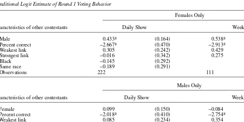
The first panel of Table 2 examines the voting behavior of women. Consistent with the descriptive evidence, women appear to be more likely to cast votes against men than against other women. This effect is quite large. Consider a daily show with six white contestants, three men, and three women, all with identical performance. The probability of a given woman voting against a particular man is 23.3 percent while the probability that she votes against a particular woman is only 15.1 percent. As shown in the Appendix, this effect disappears immediately after Round 1 in the weekly show while diminishing more slowly in the daily show. Also consistent with the descriptive evidence, the next two panels of Table 2 show that there is no indication of discrimi-nation by men against women or by whites against blacks. This holds true for all rounds of the game.
As one would expect, for all demographic groups in the early stages of the game, the higher the percentage of the questions that the player answers correctly the less likely other contestants are to cast votes against that player. However, as the game pro-gresses, the percent correct becomes less and less important. This confirms the basic logic that players have an incentive to vote against weak players in the early rounds of the game but, in the later rounds, this incentive is partially offset by the incentive to vote against stronger players.
VI. Why Women Vote Against Men
This section attempts to distinguish between the three possible hypotheses for why women are more likely to vote against men: statistical discrimi-nation, strategic discrimidiscrimi-nation, and preference-based discrimination. Here again, we primarily focus our analysis on voting behavior in Round 1.
A. The Case Against Statistical Discrimination
Recall that statistical discrimination with correct priors can take two forms. In the first, the mean performance level is different across groups. Assuming that players wish to vote off weak players in Round 1, then if statistical discrimination of this type explains women’s voting patterns, the performance of males must be on average worse than the performance of females. Table 3 documents the average percent cor-rect for males and females by round and by show type. There is virtually no differ-ence in performance levels for males and females in either show in the early rounds, while in the later rounds males actually perform better than their female counter-parts.10In addition, if men are truly worse than women at playing the game, then both
Antonovics, Arcidiacono, and Walsh 931
The Journal of Human Resources
Table 2
Conditional Logit Estimate of Round 1 Voting Behavior
Females Only
Characteristics of other contestants Daily Show Weekly Show
Male 0.433* (0.164) 0.538* (0.224)
Percent correct −2.667* (0.470) −2.913* (0.506)
Weakest link 0.305 (0.242) 0.429 (0.283)
Strongest link −0.016 (0.342) 0.275 (0.510)
Black −0.145 (0.292)
Same race −0.189 (0.291)
Observations 222 111
Males Only
Characteristics of other contestants Daily Show Weekly Show
Female 0.099 (0.150) −0.084 (0.210)
Percent correct −2.018* (0.410) −2.754* (0.488)
Weakest link 0.085 (0.234) 0.354 (0.263)
Strongest link −0.596 (0.352) −0.728 (0.746)
Black 0.199 (0.308)
Same race −0.201 (0.309)
Antono
vics, Arcidiacono, and W
alsh
933
Whites Only
Characteristics of other contestants Daily Show Weekly Show
Female −0.170 (0.124)
Same gender −0.271* (0.123)
Percent correct −2.508* (0.352)
Weakest link 0.057 (0.192)
Strongest link −0.360 (0.284)
Black 0.000 (0.144)
Observations 349
The Journal of Human Resources
Table 3
Performance by Race and Gender
Females Males Blacks Whites
Show/ Percent Standard Percent Standard Percent Standard Percent Standard
Round Sample Correct Deviation Sample Correct Deviation Sample Correct Deviation Sample Correct Deviation
Daily
1 225 0.668 0.306 225 0.667 0.340 97 0.639 0.346 353 0.675 0.317
2 186 0.630 0.341 184 0.632 0.336 79 0.657 0.325 291 0.624 0.342
3 159 0.600 0.308 141 0.614 0.337 63 0.583 0.366 237 0.613 0.309
4 115 0.580 0.353 110 0.659 0.292 48 0.647 0.334 177 0.611 0.325
Weekly
1 111 0.608 0.367 113 0.631 0.328 27 0.629 0.391 196 0.618 0.342
2 98 0.613 0.311 98 0.611 0.344 23 0.563 0.343 173 0.618 0.325
3 85 0.579 0.303 83 0.631 0.302 20 0.698 0.319 148 0.592 0.299
4 67 0.569 0.274 73 0.655 0.308 18 0.580 0.323 122 0.619 0.292
5 49 0.511 0.252 63 0.639* 0.246 12 0.636 0.277 100 0.577 0.254
6 40 0.539 0.287 44 0.548 0.236 8 0.413 0.289 76 0.558 0.254
women andmen should be more likely to vote against men in the early rounds of the game. We find no evidence of this. An analogous argument holds if players wish to vote off strong players in the first round. Hence, there is no evidence that statistical discrimination based upon differences in mean group performance is driving females to vote against males.
The second type of statistical discrimination, where the signals on ability are more informative for one group than another, is ruled out by the fact that women are dis-criminating against men rather than against women. Recall that information-based statistical discrimination implies that within-group performance is more informative than out-of-group performance. Hence, both poor performance and good performance are weighted more heavily by members of one’s own group—implying that women would be more likely to vote against women than against men. We find the exact opposite result.
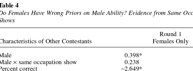
Next, we turn to the case of incorrect prior beliefs regarding group performance. It is possible that in the early rounds of the game, women have not yet learned that men perform as well as women. Our data set contains 13 episodes of the daily show in which all of the contestants have the same occupation. Should erroneous prior beliefs exist, it seems reasonable to expect that workers in the same occupation would have more informative priors on the abilities of their opposite-sex contestants than do con-testants of differing occupations. Thus, in Table 4, we reexamine women’s voting behavior in Round 1 and interact a dummy variable for the shows in which all of the contestants have the same occupation with the male indicator. Under the incorrect pri-ors hypothesis, one would expect a negative coefficient on this interaction term. However, the coefficient on this term is positive, although insignificant, providing weak evidence that women in the same occupation are more likely to vote against men than are women in different occupations. We provide additional evidence against the hypothesis of incorrect prior beliefs in our discussion of explicit collusion below.
Antonovics, Arcidiacono, and Walsh 935
Table 4
Do Females Have Wrong Priors on Male Ability? Evidence from Same Occupation Shows
Round 1 Characteristics of Other Contestants Females Only
Male 0.398* (0.178)
Male ×same occupation show 0.238 (0.472)
Percent correct −2.649* (0.471)
Weakest link 0.309 (0.243)
Strongest link −0.026 (0.342)
Black −0.139 (0.292)
Same race −0.192 (0.292)
Observations 222
Note: Conditional logit estimates of the probability of a female voting against a particular contestant. Standard errors are in parentheses.
B. The Case Against Strategic Discrimination
We now test whether women are acting cooperatively with one another. There are two basic types of collusive behavior in which women might engage: explicit collu-sion and implicit collucollu-sion. Under explicit collucollu-sion, the presumption is that the women are following some agreed upon pattern of voting. Under implicit collusion, the presumption is that women are implicitly using men as focal points for collusive behavior.
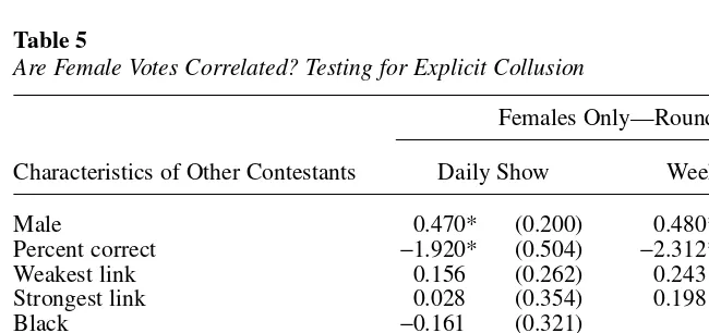
To test for explicit collusion, we include in the female Round 1 conditional logits the total votes cast for each contestant by the other contestants as well as the total votes cast by the other female contestants.11The first variable captures the fact that there may be unobservable characteristics that lead allindividuals to vote against a particular contestant. The second variable captures correlation among the votes of women—controlling for unobservable characteristics that draw the votes of all con-testants. In order for there to be explicit collusion among females, the coefficient on this latter variable, total votes cast by other women, must be positive. This is true regardless of whether it is optimal for contestants to vote off strong or weak players. Results for this specification are shown in Table 5. Importantly, the total votes cast by other women has no more predictive power than the total votes cast by men. This can be seen because once we control for the total votes cast, the coefficient on votes cast by women is small and insignificant. Hence, there is no evidence of explicit collusion.
11. We also performed this analysis for the male subsample and for Round 2 of the daily show. Gender again had no effect on the voting behavior of men and the results for Round 2 were very similar to the results from Round 2; female votes are not correlated except through total votes.
Table 5
Are Female Votes Correlated? Testing for Explicit Collusion
Females Only—Round 1
Characteristics of Other Contestants Daily Show Weekly Show
Male 0.470* (0.200) 0.480* (0.242)
Percent correct −1.920* (0.504) −2.312* (0.551)
Weakest link 0.156 (0.262) 0.243 (0.300)
Strongest link 0.028 (0.354) 0.198 (0.512)
Black −0.161 (0.321)
Same race −0.237 (0.321)
Total votes cast by
Other contestants 0.541* (0.102) 0.223 (0.120)
Other female contestants −0.054 (0.179) −0.028 (0.206)
Observations 222 111
Note: Conditional logit estimates of the probability of a female voting against a particular contestant. Standard errors are in parenthesis.
The fact that the coefficient on female votes is small and insignificant also allows us to reject many other explanations for the discriminatory behavior of women. In particular, it suggests that women are not discriminating on some unobserved charac-teristic correlated with being male as this too should have led to a positive coefficient on votes cast by women. For example, if particular men are arrogant or make poor (in the eyes of women) banking decisions, then the votes of the other women should reflect this. Instead, the results suggest that any unobservable characteristics of men that are unappealing to women are equally unappealing to men. Note that this also helps to rule out discrimination based upon bad expectations. In particular, the only bad expectations that can exist involve women expecting all men to perform equally poorly—that is, there can be no correlation between these bad expectations and any observable (to the voter, not to the researcher) characteristics.
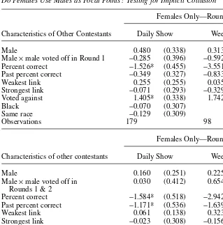
We next test whether or not women are implicitly colluding to vote off men. The first evidence that this is not the case comes from the diminishing coefficient on same sex as we move to the later rounds of the game. If implicit collusion is working, then there is no reason to stop colluding against men in the later rounds. The second indi-cation that implicit collusion is not driving the results is that implicit collusion does not appear to be reinforcing. That is, if implicit collusion successfully occurs in one round (a man is voted off), then it should be more likely to occur in the next round. Again, this prediction does not depend on whether or not the optimal strategy is to vote off strong or weak players. The top panel of Table 6 reports the conditional log-its for Round 2 of the daily and weekly shows with an indicator variable for whether a man was voted off in Round 1. Similarly, the bottom panel reports the conditional logits for Round 3 with an indicator variable for whether a man was voted off in both Round 1 and Round 2. Although not significant, three of the four interactions are neg-ative, implying that, if anything, removing males makes it less likely that women will vote off men in future rounds. Hence, we find no evidence of strategic discrimination through either implicit or explicit collusion.
These results should be interpreted with some caution. Given that there is selection into later rounds, contestants update their beliefs regarding the abilities of their oppo-nents and observe the votes of their oppooppo-nents in previous rounds. To partially con-trol for these factors, we include the cumulative percent correct from the previous rounds as well as whether the opponent had ever voted against the contestant in any of the previous rounds. The discrimination coefficients for women—and correspond-ingly the discrimination coefficients for men and for whites—are not sensitive to the inclusion of these variables.
C. The Case for Preference-Based Discrimination
The only remaining explanation is that women simply prefer playing with women. Consistent with this explanation, the coefficient on male diminishes in later rounds as the price of discriminating based upon preferences increases. Further, this coefficient falls faster in the weekly show, disappearing after one round. This is consistent with the theory of preference-based discrimination since the cost of discriminating is higher in the weekly show where the total prize money is substantially larger.
We have attempted to further test this explanation by including controls for the amount of money banked (the size of the pot) at the voting stage. If preference-based
discrimination exists, higher amounts of money banked should lead to less discrimi-nation. Estimates of models of this type were mixed, with evidence that at the lowest quartile of money banked discrimination increases (consistent with the theory) but discrimination also increases at the highest quartile of money banked (inconsistent with the theory). One possible explanation for the latter is that, in order to bank a large sum of money, every contestant needs to perform well, and if every player is similarly talented at playing the game, then there is no extra cost associated with voting against men, regardless of the amount of money banked. Unfortunately, the small sample sizes make it difficult to further test this hypothesis.
Table 6
Do Females Use Males as Focal Points? Testing for Implicit Collusion
Females Only—Round 2
Characteristics of Other Contestants Daily Show Weekly Show
Male 0.480 (0.338) 0.313 (0.418)
Male ×male voted off in Round 1 −0.285 (0.396) −0.592 (0.518)
Percent correct −1.526* (0.455) −3.551* (0.673)
Past percent correct −0.349 (0.327) −0.833* (0.422)
Weakest link 0.255 (0.255) 0.035 (0.323)
Strongest link −0.071 (0.293) −0.329 (0.786)
Voted against 1.405* (0.338) 1.742* (0.421)
Black −0.070 (0.307)
Same race −0.129 (0.309)
Observations 179 98
Females Only—Round 3
Characteristics of other contestants Daily Show Weekly Show
Male 0.160 (0.251) 0.225 (0.299)
Male ×male voted off in 0.030 (0.412) 0.654 (0.637) Rounds 1 & 2
Percent correct −1.584* (0.518) −2.942* (0.714)
Past percent correct −1.171* (0.536) −1.639* (0.694)
Weakest link 0.061 (0.138) 0.323 (0.337)
Strongest link −0.023 (0.308) −0.156 (0.600)
Voted against 1.232* (0.314) 0.904* (0.438)
Black −0.722 (0.559)
Same race −1.070 (0.556)
Observations 156 85
Antono
vics, Arcidiacono, and W
alsh
939
Table 7
Conditional Logits of Voting Behavior in the Daily Show
Characteristics of Other Contestants Round 1 Round 2 Round 3 Round 4
Females only
Male 0.433* (0.164) 0.276 (0.176) 0.170 (0.202) 0.133 (0.291)
Percent correct −2.667* (0.470) −1.538* (0.453) −1.584* (0.518) −0.775 (0.809)
Past percent correct −0.346 (0.327) −1.175 (0.533) −0.453 (0.913)
Weakest link 0.305 (0.242) 0.246 (0.253) 0.060 (0.138) 0.195 (0.380)
Strongest link −0.016 (0.342) −0.070 (0.293) −0.022 (0.307) 0.405 (0.340)
Voted against 1.402* (0.338) 1.232* (0.314) 1.232* (0.439)
Black −0.145 (0.292) −0.065 (0.307) −0.718 (0.557) −0.798 (0.585)
Same race −0.189 (0.291) −0.127 (0.308) −1.067 (0.555) −1.322* (0.596)
Observations 222 179 156 113
Males only
Female 0.099 (0.150) −0.09 (0.171) 0.278 (0.236) −0.056 (0.281)
Percent correct −2.018* (0.410) −1.843* (0.445) −2.289* (0.625) −0.786 (0.809)
Past percent correct −0.493 (0.343) −0.761 (0.550) −0.486 (0.944)
Weakest link 0.085 (0.234) −0.033 (0.250) 0.024 (0.173) 0.188 (0.366)
Strongest link −0.596 (0.352) −0.395 (0.320) −0.191 (0.360) 0.232 (0.367)
The Journal of Human Resources
Table 7 (continued)
Characteristics of Other Contestants Round 1 Round 2 Round 3 Round 4
Voted against 1.369* (0.307) 1.106* (0.341) 0.899* (0.419)
Black −0.199 (0.308) −0.026 (0.314) −0.347 (0.453) −0.504 (0.484)
Same race −0.201 (0.309) 0.033 (0.317) 0.188 (0.453) −0.303 (0.489)
Observations 222 179 138 110
Whites only
Female −0.170 (0.124) −0.161 (0.138) 0.007 (0.167) −0.290 (0.228)
Same gender −0.271* (0.123) −0.131 (0.138) −0.241 (0.165) 0.118 (0.217)
Percent correct −2.508* (0.352) −1.918* (0.359) −1.765* (0.473) −0.605 (0.624)
Past percent correct −0.589* (0.266) −0.863* (0.415) −0.320 (0.734)
Weakest link 0.057 (0.192) −0.076 (0.202) −0.025 (0.161) 0.245 (0.304)
Strongest link −0.360 (0.284) 0.006 (0.234) −0.214 (0.255) 0.295 (0.270)
Black 0.000 (0.144) −0.012 (0.165) −0.053 (0.200) 0.107 (0.266)
Voted against 1.433* (0.253) 1.192* (0.255) 1.170* (0.336)
Note: Conditional logit estimates of the probability of an individual voting for a particular contestant. Past percent correct is the cumulative percent correct in the previous rounds. Voted against is whether the opponent ever voted against the contestant in any of the previous rounds. Standard errors are in parenthesis.
Antono
vics, Arcidiacono, and W
alsh
941
Table 8
Conditional Logits of Voting Behavior in the Weekly Shows
Characteristics of Other
Contestants Round 1 Round 2 Round 3 Round 4 Round 5 Round 6
Females only
Male 0.538* (0.224) −0.060 (0.246) 0.371 (0.265) 0.005 (0.302) 0.665 (0.408) −0.994 (0.746) Percent correct −2.913* (0.506) −3.612* (0.672) −2.960* (0.710) 0.088 (0.785) 0.071 (1.097) 1.213 (1.895)
Past percent — —
Correct −0.853* (0.420) 1.503* (0.673) 2.329* (1.050) −1.050 (1.381) 5.499 (3.286) Weakest link 0.429 (0.283) −0.007 (0.317) 0.328 (0.339) 0.952* (0.401) 0.256 (0.469) 2.204* (0.931) Strongest link 0.275 (0.510) −0.325 (0.787) −0.155 (0.597) −1.045 (0.535) −0.500 (0.487) 0.227 (0.653) Voted against 1.774* (0.420) 0.922* (0.436) 1.168* (0.387) 1.633* (0.606) .035* (1.163)
Observations 111 98 85 66 49 39
Males only
Female −0.084 (0.210) 0.155 (0.243) 0.453 (0.269) −0.117 (0.321) −0.559 (0.320) −0.488 (0.504) Percent correct −2.754* (0.488) −2.818* (0.606) −2.560* (0.700) −2.476* (0.855) −0.087 (1.177) 1.535 (1.549)
Past percent —
Correct −1.538 (0.448) −2.167* (0.717) 2.845* (1.092) 0.190 (1.245) 1.627 (2.521) Weakest link 0.354 (0.263) −0.027 (0.330) 0.383 (0.319) 0.311 (0.343) 0.357 (0.426) 1.300* (0.625) Strongest link −0.728 (0.746) −34.200 — −0.293 (0.655) −0.712 (0.611) −0.227 (0.444) 0.286 (0.579) Voted against 1.192 (0.431) 0.359 (0.433) 1.292* (0.460) 1.136* (0.386) 0.115 (0.567)
Observations 113 98 83 71 63 42
Note: Conditional logit estimates of the probability of an individual voting for a particular contestant. Past percent correct is the cumulative percent correct in the previous rounds. Voted against is whether the opponent ever voted against the contestant in any of the previous rounds. No males voted for the strongest link in Round 2 of the weekly show. Standard errors are in parenthesis.
VII. Discussion
Given that we are interested in learning about labor market discrimi-nation, it is important to confirm that our findings are consistent with what we observe in other contexts. A number of recent audit studies (for example, Goldin and Rouse 2000 and Bertrand and Mullanaithan 2004) have documented evidence of discrimi-nation against women and blacks. We find no evidence of discrimidiscrimi-nation against these groups.
There are a number of explanations for this discrepancy. First, the contestants on the The Weakest Link operate under the scrutiny of a much larger audience than employers in the labor market. Thus, if there is a social stigma associated with dis-crimination (of any kind), then individuals may not be willing to discriminate when their actions are publicly observable. This suggests that open hiring policies may reduce discrimination. To our knowledge there has been no previous research on the impact of audiences on discriminatory behavior.
Second, as Table 3 shows, there are no significant performance differences between men and women or between blacks and whites in either the first or the second moment of the ability distribution. As a result, even if statistical discrimination is an important feature of the labor market, it would be unlikely to appear in our analysis. Thus, one interpretation of the fact that we find no evidence of discrimination against either blacks or women in our data is as support for the role of statistical discrimination in the discriminatory patterns found in recent studies of the labor market.
Somewhat surprisingly, we also find evidence that women have discriminatory preferences against men. There are a number of possible explanations for this type of behavior. First, women may dislike certain aspects of how men play the game.12
Women may also feel more compassionate toward women than toward men, and women may not like playing with men because they fear that they will not compete as well against men in the later rounds of the game. In experimental settings, Gneezy, Niederle and Rustichini (2003) and Gneezy and Rustichini (2004), for example, find evidence that competition improves the performance of men but does not do so for women.
Evidence from other settings supports the notion that women might give prefer-ential treatment to other women. As discussed previously, Dillingham, Ferber, Hamermesh (1994) find that women discriminate in favor of women in voting for offi-cers in a professional association. There is also evidence that, all else equal, women are more likely to vote for women in political contests. For example, in her analysis of voting behavior during the 1992 U.S. election, Dolan (1998) finds that women were more likely than men to vote for women candidates, even after controlling for a num-ber of ideological, issue, and party concerns. Similar results are reported by Smith and Fox (2001) for open seat house races between 1988 and 1992. Further, these authors find candidate sex does not matter to male voters once controls for other factors are
Antonovics, Arcidiacono, and Walsh 943
included. Finally, Derose et al. (2001) examine the relationship between patient satis-faction and the gender of emergency department physicians. They find that even after controlling for the patient’s age, health status, literacy level, and a number of other covariates, women gave significantly higher performance ratings to female physi-cians. Men’s satisfaction, on the other hand, was not associated with physician gen-der. While beyond the scope of this paper, understanding more about the sources of women’s preferences toward women is clearly an intriguing area for future research.
VIII. Conclusion
Understanding the nature of discrimination and its contribution to both racial and gender earnings inequality involves tackling two questions. First, we would like to know whether individuals discriminate. Second, we would like to know why individuals discriminate. In this paper we attempt to address both of these ques-tions by examining the voting behavior of contestants in The Weakest Link. Although the game show environment is clearly different from that of the labor market, diffi-culties associated with evaluating discrimination directly within the labor market motivate an analysis of behavior in more stylized settings. This research builds on the emerging experimental literature on discrimination and provides an opportunity to consider individual behavior in a high-stakes environment.
Interestingly, we find no evidence of either preference-based or strategic discrimi-nation against either blacks or women. Statistical discrimidiscrimi-nation was ruled out in The Weakest Linkin part because of the lack of performance differences across racial and gender lines. However, this may not be the case in the labor market and points toward statistical discrimination as a possible explanation for the discriminatory patterns against these groups found in a number of recent studies. In addition, we find that women discriminate against men in the early rounds of both the daily and weekly shows. The one theory consistent with the observed voting trends is preference-based discrimination. In other words, it appears that women simply prefer playing with women rather than with men. Finally, our paper suggests the need for future studies that examine the impact of audiences on discriminatory behavior.
Appendix
Here we present a simple model of statistical discrimination and discuss its implica-tions for voting behavior in the first round of The Weakest Link. An essential feature of the model is that players base their voting decisions on an indicator of player abil-ity, x, that approximates true ability, θ.
Below, we develop the implications of this simple model. In particular, we first examine voting behavior when players correctly perceive that there are real group dif-ferences in average ability. Second, we examine voting behavior when players are bet-ter able to assess the ability signals of contestants from their own group. Finally, we consider what happens if players have incorrect prior beliefs about the distribution of
θ. Interestingly, the model’s empirical predictions do not depend on whether contest-ants wish to vote off strong players or weak players.
A. Baseline Model
In this model, contestants make inferences about θgiven xusing Bayes’s Rule. Under our assumptions, the posterior distribution of θfor a contestant from group jwith first round performance xis known to be normal with mean mjand variance sj, where
( )
mj=s xj + 1-sj nj
and
.
sj j
j
2 2
2
= + v v
v
f
Note that mjis a weighted average of the player’s Round 1 performance, x, and the prior mean, µj, where the weights depend on how diffuse is the prior on θand how informative is the signal x.
B. Real Group Differences in Average Ability
Suppose that contestants from Group Ahave higher average ability than contestants from Group B, but the prior variance of θis the same for both groups. That is, sup-pose that µA> µBand σA2= σB2. In this case it is clear that, given identical signals (realizations of x), mAwill be greater than mB. Thus, if contestants wish to vote off weak players, then contestants will be more likely to vote off members of Group A than Group Band if contestants wish to vote off strong players, contestants will be more likely to vote off members of Group Bthan Group A. In either case, the central prediction is that contestants from allgroups will be more likely to vote against mem-bers of a single group. In addition, to the extent that we are able to observe x, we also should observe average group differences in performance.
C. Asymmetric Information
Now suppose instead that contestants from Group A and Group B have the same aver-age ability, but contestants are better at assessing the ability of contestants from their own group than they are of those from another group. For example, this would be the case if women (men) are better able to identify the types of questions that women (men) should be able to answer correctly. In the context of the model, we assume that
Antonovics, Arcidiacono, and Walsh 945
clear that sjis higher for members of a participant’s own group than for members of another group—implying that the posterior mean of θwill depend more heavily on x for contestants from a players own group than it will for contestants from another group. Thus, players with both the highest and the lowest posterior mean ability will be from the contestant’s own group. As a result, contestants will be more likely to vote against members of their own group than against contestants from another group, regardless of whether it is optimal for contestants to vote off strong or weak players.
D. Incorrect Prior Beliefs
Typically in models of statistical discrimination it is assumed that people have correct prior beliefs about the distribution of true ability. However, it may be possible that contestants on this program have inaccurate prior beliefs. For example, even if the dis-tribution of θis identical for men and women, women may incorrectly perceive that men are worse at playing the game than women. Since these beliefs are incorrect, they are naturally hard to verify. However, if incorrect priors explain discrimination, we would expect to see more accurate prior beliefs—and hence less discrimination—in games in which all contestants are drawn from the same occupation.
References
Aigner, Dennis, and Glen Cain. 1977. “Statistical Theories of Discrimination in the Labor
Market.” Industrial and Labor Relations Review30(2):175–87.
Altonji, Joseph, and Rebecca Blank. 1999. “Race and Gender in the Labor Market.” In
Handbook of Labor Economics, 3c, ed. Orley Ashenfelter and David Card, 3143–59. New York: Elsevier.
Altonji, Joseph, and Charles Pierret. 2001. “Employer Learning and Statistical
Discrimination.” Quarterly Journal of Economics116(1):313–50.
Anderson, Donna, and Michael Haupert. 1999. “Employment and Statistical Discrimination:
A Hands-On Experiment.” The Journal of Economics25(1):85–102.
Arrow, Kenneth. 1973. “The Theory of Discrimination.” In Discrimination in Labor Markets,
ed. Orley Ashenfelter and Albert Rees, 3–33. Princeton: Princeton University Press. Ashenfelter, Orley, and Timothy Hannan. 1986. “Sex Discrimination and Market Competition:
The Case of the Banking Industry.” Quarterly Journal of Economics101(1):149–74.
Ball, Sheryl, Catherine Eckel, Phillip Grossman, and William Zame. 2001. “Status in
Markets.” Quarterly Journal of Economics116(1):161–88.
Ball, Sheryl, and Catherine Eckel. 2003. “Stars Upon Thars.” Working Paper.
Becker, Gary. 1957. The Economics of Discrimination. Chicago: The University of Chicago
Press.
Bennet, Randall, and Kent Hickman. 1993. “Rationality and the Price is Right.” Journal of
Economic Behavior and Organization21(1):99–105.
Berk, Jonathon, Eric Hughson, and Kirk Vandezande. 1996. “The Price is Right, But Are the
Bids? An Investigation of Rational Decision Theory.” American Economic Review
86(4):954–70.
Bertrand, Marianne, and Sendhil Mullainathan. 2004. “Are Emily and Brendan More Employable than Lakisha and Jamal? A Field Experiment on Labor Market
Discrimination.” American Economic Review94(4):991–1013.
Coate, Stephen, and Glenn Loury. 1993. “Will Affirmative Action Eliminate Negative
Cross, Harry, Genvieve Kenney, Jane Mell, and Wendy Zimmerman. 1990. Employer Hiring Practices: Differential Treatment of Anglo and Hispanic Job Seekers. Washington, D.C.: Urban Institute Press.
Davis, Douglass. 1987. “Maximal Quality Selection and Discrimination in Employment.”
Journal of Economic Behavior and Organization8(1):97–112.
Derose, Kathryn, Ronald Hays, Dan McCaffrey, and David Baker. 2001. “Does Physician Gender Affect Satisfaction of Men and Women Visiting the Emergency Department?”
Journal of General Internal Medicine16(4):218–26.
Dillingham, Alan, Marianne Ferber, and Daniel Hamermesh. 1994. “Gender Discrimination
by Gender: Voting in a Professional Society.” Industrial and Labor Relations Review
47(4):622–33.
Dolan, Kathleen. 1998. “Voting for Women in the Year of the Woman.” American Journal of
Political Science42(1):272–93.
Fershtman, Chaim, and Uri Gneezy. 2001. “Discrimination in a Segmented Society: An
Experimental Approach.” Quarterly Journal of Economics116(1):351–77.
Fryer, Roland, Jacob Goeree, and Charles Holt. 2005. “Classroom Games: Experienced-Based
Discrimination.” Journal of Economic Education. Forthcoming.
Gaines, Brian. 2003. “Trueling for Dollars: Theory and Empirics of Final-Round Voting on
The Weakest Link.” Working Paper.
Gertner, Robert. 1993. “Game Shows and Economic Behavior: Risk Taking on ‘Card
Sharks’.” Quarterly Journal of Economics108(2):507–21.
Gilbert, George, and Rhonda Hatcher. 1994. “Wagering in Final Jeopardy!” Mathematics
Magazine67(4):268–77.
Gneezy, Uri, and Aldo Rustichini. 2004. “Gender and Competition at a Young Age.”
American Economic Review94(2):377–81.
Gneezy, Uri, Muriel Niederle, and Aldo Rustichini. 2003. “Performance in Competitive
Environments: Gender Differences.” Quarterly Journal of Economics118(3):1049–74.
Goldin, Claudia, and Cecilia Rouse. 2000. “Orchestrating Impartiality: The Impact of “Blind”
Auditions on Female Musicians.” American Economic Review90(4):715–41.
Heckman, James. 1998. “Detecting Discrimination.” Journal of Economic Perspectives
12(1):101–16.
Heckman, James, and Peter Siegelman. 1992. “The Urban Institute Audit Studies: Their
Methods and Findings.” In Clear and Convincing Evidence: Measurement of
Discrimination in America, ed. Michael Fix and Raymond Struyk, 187–258. Washington, D.C.: Urban Institute Press.
Hellerstein, Judith, David Neumark, and Kenneth Troske. 2002. “Market Forces and Sex
Discrimination.” Journal of Human Resources37(2):353–80.
Holm, Hakan. 2000. “Gender-Based Focal Points.” Games and Economic Behavior
32(2):292–314.
Kahn, Lawrence, and Peter Sherer. 1988. “Racial Differences in Professional Basketball
Players’ Compensation.” Journal of Labor Economics6(1):40–61.
Levitt, Steven. 2004. “Testing Theories of Discrimination: Evidence from The Weakest Link.”
Journal of Law and Economics47(2):431–52.
Lundberg, Shelly, and Richard Startz. 1983. “Private Discrimination and Social Intervention
in a Competitive Labor Market.” The American Economic Review73(3):340–47.
Mason, Charles, Owen Phillips, and Douglass Reddington. 1991. “The Role of Gender in
Non-Cooperative Games.” Journal of Economic Behavior and Organization15(2):
215–335.
Metrick, Andrew. 1995. “A Natural Experiment in Jeopardy!” American Economic Review
85(1):240–53.