3
Exponential Family and Generalized
Linear Models
3.1 Introduction
Linear models of the form
E(Yi) =µi =xTiβ; Yi∼N(µi, σ2) (3.1)
where the random variables Yi are independent are the basis of most analyses of continuous data. The transposed vectorxTi represents theith row of the design matrix X. The example about the relationship between birth-weight and gestational age is of this form, see Section 2.2.2. So is the exercise on plant growth where Yi is the dry weight of plants and Xhas elements to identify the treatment and control groups (Exercise 2.1). Generalizations of these examples to the relationship between a continuous response and several explanatory variables (multiple regression) and comparisons of more than two means (analysis of variance) are also of this form.
Advances in statistical theory and computer software allow us to use meth-ods analogous to those developed for linear models in the following more general situations:
1. Response variables have distributions other than the Normal distribution – they may even be categorical rather than continuous.
2. Relationship between the response and explanatory variables need not be of the simple linear form in (3.1).
One of these advances has been the recognition that many of the ‘nice’ properties of the Normal distribution are shared by a wider class of distribu-tions called the exponential family of distributions. These distributions and their properties are discussed in the next section.
A second advance is the extension of the numerical methods to estimate the parameters β from the linear model described in (3.1) to the situation where there is some non-linear function relating E(Yi) =µi to the linear component
xTiβ, that is
g(µi) =xTi β
com-putation involving numerical optimization of non-linear functions. Procedures to do these calculations are now included in many statistical programs.
This chapter introduces the exponential family of distributions and defines generalized linear models. Methods for parameter estimation and hypothesis testing are developed in Chapters 4 and 5, respectively.
3.2 Exponential family of distributions
Consider a single random variable Y whose probability distribution depends on a single parameterθ. The distribution belongs to the exponential family if it can be written in the form
f(y;θ) =s(y)t(θ)ea(y)b(θ) (3.2)
wherea,b,sand tare known functions. Notice the symmetry betweeny and θ. This is emphasized if equation (3.2) is rewritten as
f(y;θ) = exp[a(y)b(θ) +c(θ) +d(y)] (3.3)
where s(y) = expd(y) and t(θ) = expc(θ).
If a(y) =y, the distribution is said to be in canonical (that is, standard)
form and b(θ) is sometimes called the natural parameter of the distribu-tion.
If there are other parameters, in addition to the parameter of interest θ, they are regarded as nuisance parameters forming parts of the functions a, b,c and d, and they are treated as though they are known.
Many well-known distributions belong to the exponential family. For exam-ple, the Poisson, Normal and binomial distributions can all be written in the canonical form – see Table 3.1.
3.2.1 Poisson distribution
The probability function for the discrete random variable Y is
f(y, θ) = θ ye−θ
y!
Table 3.1 Poisson, Normal and binomial distributions as members of the exponential family.
Distribution Natural parameter c d
Poisson logθ −θ −logy!
Normal µ
σ2 −
µ2 2σ2 −
1 2log
2πσ2
− y 2
2σ2
Binomial log
π 1−π
nlog (1−π) logny
where y takes the values 0,1,2, . . . . This can be rewritten as
f(y, θ) = exp(ylogθ−θ−logy!)
which is in the canonical form because a(y) =y. Also the natural parameter is logθ.
The Poisson distribution, denoted by Y ∼ P oisson(θ), is used to model count data. Typically these are the number of occurrences of some event in a defined time period or space, when the probability of an event occurring in a very small time (or space) is low and the events occur independently. Exam-ples include: the number of medical conditions reported by a person (Example 2.2.1), the number of tropical cyclones during a season (Example 1.6.4), the number of spelling mistakes on the page of a newspaper, or the number of faulty components in a computer or in a batch of manufactured items. If a random variable has the Poisson distribution, its expected value and variance are equal. Real data that might be plausibly modelled by the Poisson distri-bution often have a larger variance and are said to be overdispersed, and the model may have to be adapted to reflect this feature. Chapter 9 describes various models based on the Poisson distribution.
3.2.2 Normal distribution
The probability density function is
f(y;µ) = 1
(2πσ2)1/2exp
−2σ12(y−µ)2
where µis the parameter of interest and σ2 is regarded as a nuisance param-eter. This can be rewritten as
f(y;µ) = exp other terms in (3.3) are
c(µ) =− µ
worthwhile trying to identify a transformation, such asy′ = logy ory′=√y,
which produces datay′ that are approximately Normal.
3.2.3 Binomial distribution
Consider a series of binary events, called ‘trials’, each with only two possible outcomes: ‘success’ or ‘failure’. Let the random variable Y be the number of ‘successes’ in n independent trials in which the probability of success, π, is the same in all trials. Then Y has the binomial distribution with probability density function
f(y;π) =
n y
πy(1−π)n−y
whereytakes the values 0,1,2, . . . , n. This is denoted byY ∼binomial(n, π). Hereπis the parameter of interest and nis assumed to be known. The prob-ability function can be rewritten as
f(y;µ) = exp
ylogπ−ylog(1−π) +nlog(1−π) + log
n y
which is of the form (3.3) with b(π) = logπ−log(1−π) = log [π/(1−π)]. The binomial distribution is usually the model of first choice for observa-tions of a process with binary outcomes. Examples include: the number of candidates who pass a test (the possible outcomes for each candidate being to pass or to fail), or the number of patients with some disease who are alive at a specified time since diagnosis (the possible outcomes being survival or death).
Other examples of distributions belonging to the exponential family are given in the exercises at the end of the chapter; not all of them are of the canonical form.
3.3 Properties of distributions in the exponential family
We need expressions for the expected value and variance ofa(Y). To find these we use the following results that apply for any probability density function provided that the order of integration and differentiation can be interchanged. From the definition of a probability density function, the area under the curve is unity so
f(y;θ)dy= 1 (3.4)
where integration is over all possible values of y. (If the random variableY is discrete then integration is replaced by summation.)
If we differentiate both sides of (3.4) with respect to θ we obtain d
dθ
f(y;θ)dy= d
dθ.1 = 0 (3.5)
If the order of integration and differentiation in the first term is reversed
then (3.5) becomes
df(y;θ)
dθ dy= 0 (3.6)
Similarly if (3.4) is differentiated twice with respect to θ and the order of integration and differentiation is reversed we obtain
d2f(y;θ)
dθ2 dy= 0. (3.7)
These results can now be used for distributions in the exponential family. From (3.3)
f(y;θ) = exp [a(y)b(θ) +c(θ) +d(y)]
so
df(y;θ)
dθ = [a(y)b
′(θ) +c′(θ)]f(y;θ).
By (3.6)
[a(y)b′(θ) +c′(θ)]f(y;θ)dy= 0.
This can be simplified to
b′(θ)E[a(y)] +c′(θ) = 0 (3.8)
because
a(y)f(y;θ)dy =E[a(y)] by the definition of the expected value and
c′(θ)f(y;θ)dy=c′(θ) by (3.4). Rearranging (3.8) gives
E[a(Y)] =−c′(θ)/b′(θ). (3.9)
A similar argument can be used to obtain var[a(Y)].
d2f(y;θ)
dθ2 = [a(y)b′′(θ) +c′′(θ)]f(y;θ) + [a(y)b′(θ) +c′(θ)] 2
f(y;θ) (3.10)
The second term on the right hand side of (3.10) can be rewritten as
[b′(θ)]2{a(y)−E[a(Y)]}2f(y;θ) using (3.9). Then by (3.7)
d2f(y;θ)
dθ2 dy=b
′′(θ)E[a(Y)] +c′′(θ) + [b′(θ)]2var[a(Y)] = 0 (3.11) because
{a(y)−E[a(Y)]}2f(y;θ)dy= var[a(Y)] by definition. Rearranging (3.11) and substituting (3.9) gives
var[a(Y)] = b′′(θ)c′(θ)−c′′(θ)b′(θ)
[b′(θ)]3 (3.12)
We also need expressions for the expected value and variance of the deriva-tives of the log-likelihood function. From (3.3), the log-likelihood function for a distribution in the exponential family is
l(θ;y) =a(y)b(θ) +c(θ) +d(y).
The derivative of l(θ;y) with respect toθ is
U(θ;y) = dl(θ;y)
dθ =a(y)b
′(θ) +c′(θ).
The functionU is called the score statisticand, as it depends ony,it can be regarded as a random variable, that is
U =a(Y)b′(θ) +c′(θ). (3.13)
Its expected value is
E(U) =b′(θ)E[a(Y)] +c′(θ).
From (3.9)
E(U) =b′(θ)
−c
′(θ)
b′(θ) +c
′(θ) = 0. (3.14)
The variance ofU is called theinformationand will be denoted byI.
Us-ing the formula for the variance of a linear transformation of random variables (see (1.3) and (3.13))
I= var(U) =b′(θ)2
var[a(Y)].
Substituting (3.12) gives
var(U) = b
′′(θ)c′(θ)
b′(θ) −c
′′(θ). (3.15)
The score statistic U is used for inference about parameter values in gen-eralized linear models (see Chapter 5).
Another property of U which will be used later is
var(U) = E(U2) =−E(U′). (3.16)
The first equality follows from the general result
var(X) = E(X2)−[E(X)]2
for any random variable, and the fact that E(U) = 0 from (3.14). To obtain the second equality, we differentiateU with respect toθ; from (3.13)
U′= dU
dθ =a(Y)b
′′(θ) +c′′(θ).
Therefore the expected value ofU′ is
E(U′) = b′′(θ)E[a(Y)] +c′′(θ)
= b′′(θ)
−c′(θ)
b′(θ) +c
′′(θ) (3.17)
= −var(U) =−I
by substituting (3.9) and then using (3.15).
3.4 Generalized linear models
The unity of many statistical methods was demonstrated by Nelder and Wed-derburn (1972) using the idea of a generalized linear model. This model is defined in terms of a set of independent random variables Y1, . . . , YN each with a distribution from the exponential family and the following properties:
1. The distribution of eachYihas the canonical form and depends on a single parameterθi (theθi’s do not all have to be the same), thus
f(yi;θi) = exp [yibi(θi) +ci(θi) +di(yi)].
2. The distributions of all the Yi’s are of the same form (e.g., all Normal or all binomial) so that the subscripts onb,c andd are not needed.
Thus the joint probability density function of Y1, . . . , YN is
The parameters θi are typically not of direct interest (since there may be one for each observation). For model specification we are usually interested in a smaller set of parameters β1, . . . , βp (where p < N ). Suppose that E(Yi) = µi where µi is some function of θi. For a generalized linear model there is a transformation of µi such that
g(µi) =xTi β.
In this equation
g is a monotone, differentiable function called the link function; xi is a
p ×1 vector of explanatory variables (covariates and dummy variables for levels of factors),
ith column of the design matrix X.
1. Response variables Y1, . . . , YN which are assumed to share the same dis-tribution from the exponential family;
2. A set of parameters β and explanatory variables
X=
3. A monotone link function g such that
g(µi) =xTiβ
where
µi = E(Yi).
This chapter concludes with three examples of generalized linear models.
3.5 Examples
3.5.1 Normal Linear Model
The best known special case of a generalized linear model is the model
E(Yi) =µi=xTiβ; Yi∼N(µi, σ2)
whereY1, ..., YN are independent. Here the link function is the identity func-tion,g(µi) =µi. This model is usually written in the form
⎦ and the ei’s are independent, identically distributed
ran-dom variables withei∼N(0, σ2) for i= 1, ..., N.
In this form, the linear component µ = Xβ represents the ‘signal’ and e
represents the ‘noise’, random variation or ‘error’. Multiple regression, analysis of variance and analysis of covariance are all of this form. These models are considered in Chapter 6.
3.5.2 Historical Linguistics
Consider a language which is the descendent of another language; for example, modern Greek is a descendent of ancient Greek, and the Romance languages are descendents of Latin. A simple model for the change in vocabulary is that if the languages are separated by time t then the probability that they have cognate words for a particular meaning is e−θt where θ is a parameter (see
Figure 3.1). It is believed thatθis approximately the same for many commonly used meanings. For a test list ofN different commonly used meanings suppose that a linguist judges, for each meaning, whether the corresponding words in
Latin word
Modern French word
Modern Spanish word
time
Figure 3.1 Schematic diagram for the example on historical linguistics.
two languages are cognate or not cognate. We can develop a generalized linear model to describe this situation.
Define random variables Y1, . . . , YN as follows:
Yi=
1 if the languages have cognate words for meaningi, 0 if the words are not cognate.
Then
P(Yi= 1) =e−θt and
P(Yi = 0) = 1−e−θt.
This is a special case of the distributionbinomial(n, π) withn= 1 and E(Yi) =
π=e−θt. In this case the link functiong is taken as logarithmic
g(π) = logπ=−θt
so that g[E(Y)] is linear in the parameter θ. In the notation used above,
xi= [−t] (the same for all i) and β= [θ].
3.5.3 Mortality Rates
For a large population the probability of a randomly chosen individual dying at a particular time is small. If we assume that deaths from a non-infectious disease are independent events, then the number of deaths Y in a population can be modelled by a Poisson distribution
f(y;µ) = µ ye−µ
y!
where ycan take the values 0,1,2, . . . andµ= E(Y) is the expected number of deaths in a specified time period, such as a year.
The parameterµwill depend on the population size, the period of observa-tion and various characteristics of the populaobserva-tion (e.g., age, sex and medical history). It can be modelled, for example, by
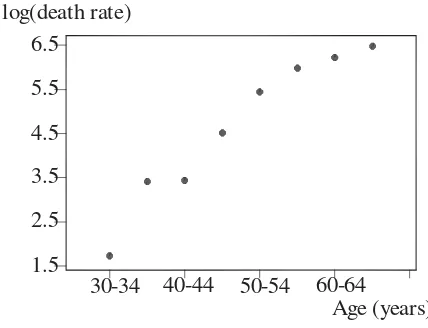
Table 3.2 Numbers of deaths from coronary heart disease and population sizes by 5-year age groups for men in the Hunter region of New South Wales, Australia in 1991.
Age group Number of Population Rate per 100,000 men
(years) deaths, yi size,ni per year,yi/ni×10,000
30 - 34 1 17,742 5.6
35 - 39 5 16,554 30.2
40 - 44 5 16,059 31.1
45 - 49 12 13,083 91.7
50 - 54 25 10,784 231.8
55 - 59 38 9,645 394.0
60 - 64 54 10,706 504.4
65 - 69 65 9,933 654.4
30-34 40-44 50-54 60-64 1.5
2.5 3.5 4.5 5.5 6.5
Age (years) log(death rate)
Figure 3.2 Death rate per 100,000 men (on a logarithmic scale) plotted against age.
wherenis the population size and λ(xTβ) is the rate per 100,000 people per year (which depends on the population characteristics described by the linear componentxTβ).
Changes in mortality with age can be modelled by taking independent ran-dom variablesY1, . . . , YN to be the numbers of deaths occurring in successive age groups. For example, Table 3.2 shows age-specific data for deaths from coronary heart disease.
Figure 3.2shows how the mortality rateyi/ni×100,000 increases with age. Note that a logarithmic scale has been used on the vertical axis. On this scale the scatter plot is approximately linear, suggesting that the relationship between yi/ni and age group i is approximately exponential. Therefore a
possible model is
E(Yi) =µi=nieθi ; Yi∼P oisson(µi),
where i= 1 for the age group 30-34 years, i= 2 for 35-39, ..., i= 8 for 65-69 years.
This can be written as a generalized linear model using the logarithmic link function
g(µi) = logµi = logni+θi
which has the linear componentxTiβ withxTi =
logni i
andβ=
1 θ .
3.6 Exercises
3.1 The following relationships can be described by generalized linear models. For each one, identify the response variable and the explanatory variables, select a probability distribution for the response (justifying your choice) and write down the linear component.
(a) The effect of age, sex, height, mean daily food intake and mean daily energy expenditure on a person’s weight.
(b) The proportions of laboratory mice that became infected after exposure to bacteria when five different exposure levels are used and 20 mice are exposed at each level.
(c) The relationship between the number of trips per week to the super-market for a household and the number of people in the household, the household income and the distance to the supermarket.
3.2 If the random variable Y has the Gamma distribution with a scale pa-rameterθ,which is the parameter of interest, and a known shape parameter φ, then its probability density function is
f(y;θ) = y
φ−1θφe−yθ
Γ(φ) .
Show that this distribution belongs to the exponential family and find the natural parameter. Also using results in this chapter, find E(Y) and var(Y). 3.3 Show that the following probability density functions belong to the
expo-nential family:
(a) Pareto distributionf(y;θ) =θy−θ−1. (b) Exponential distributionf(y;θ) =θe−yθ.
(c) Negative binomial distribution
f(y;θ) =
y+r−1 r−1
θr(1−θ)y
3.4 Use results (3.9) and (3.12) to verify the following results:
(a) For Y ∼P oisson(θ), E(Y) = var(Y) =θ. (b) For Y ∼N(µ, σ2), E(Y) =µ and var(Y) =σ2.
(c) For Y ∼binomial(n, π), E(Y) =nπ and var(Y) =nπ(1−π).
3.5 Do you consider the model suggested in Example 3.5.3 to be adequate for the data shown in Figure 3.2? Justify your answer. Use simple linear regression (with suitable transformations of the variables) to obtain a model for the change of death rates with age. How well does the model fit the data? (Hint: compare observed and expected numbers of deaths in each groups.)
3.6 Consider N independent binary random variablesY1, . . . , YN with
P(Yi= 1) =πi andP(Yi= 0) = 1−πi .
The probability function ofYi can be written as
πyi
i (1−πi) 1−yi
whereyi = 0 or 1.
(a) Show that this probability function belongs to the exponential family of distributions.
(b) Show that the natural parameter is
log
πi 1−πi
.
This function, the logarithm of theodds πi/(1−πi), is called thelogit function.
(c) Show that E(Yi) =πi. (d) If the link function is
g(π) = log
π 1−π
=xTβ
show that this is equivalent to modelling the probabilityπ as
π= e
xTβ
1 +exTβ.
(e) In the particular case wherexTβ=β1+β2x, this gives
π= e
β1+β2x
1 +eβ1+β2x
which is the logistic function.
(f) Sketch the graph of π against x in this case, taking β1 and β2 as con-stants. How would you interpret this graph if x is the dose of an insec-ticide andπ is the probability of an insect dying?
3.7 Is theextreme value (Gumbel)distribution, with probability density function
f(y;θ) = 1 φexp
(y−θ)
φ −exp
(y−θ) φ
(whereφ >0 regarded as a nuisance parameter) a member of the exponen-tial family?
3.8 SupposeY1, ..., YN are independent random variables each with the Pareto distribution and
E(Yi) = (β0+β1xi)2.
Is this a generalized linear model? Give reasons for your answer. 3.9 Let Y1, . . . , YN be independent random variables with
E(Yi) =µi=β0+ log (β1+β2xi) ; Yi∼N(µ, σ2)
for alli= 1, ..., N. Is this a generalized linear model? Give reasons for your answer.
3.10 For the Pareto distribution find the score statistics U and the information