EURACHEM / CITAC Guide
Quantifying Uncertainty in
Analytical Measurement
Second Edition
EURACHEM/CITAC Guide
Quantifying Uncertainty in
Analytical Measurement
Second Edition
Editors
S L R Ellison (LGC, UK)
M Rosslein (EMPA, Switzerland) A Williams (UK)
Composition of the Working Group
EURACHEM members A Williams Chairman UK
S Ellison Secretary LGC, Teddington, UK
M Berglund Institute for Reference Materials and Measurements, Belgium
W Haesselbarth Bundesanstalt fur Materialforschung und Prufung, Germany
K Hedegaard EUROM II
R Kaarls Netherlands Measurement Institute, The Netherlands
M Månsson SP Swedish National Testing and Research Institute, Sweden
M Rösslein EMPA St. Gallen, Switzerland
R Stephany National Institute of Public Health and the Environment, The Netherlands
A van der Veen Netherlands Measurement Institute, The Netherlands
W Wegscheider University of Mining and Metallurgy, Leoben, Austria
H van de Wiel National Institute of Public Health and the Environment, The Netherlands
R Wood Food Standards Agency, UK
CITAC Members
Pan Xiu Rong Director, NRCCRM,. China
M Salit National Institute of Science and Technology USA
A Squirrell NATA, Australia
K Yasuda Hitachi Ltd, Japan
AOAC Representatives
R Johnson Agricultural Analytical Services, Texas State Chemist, USA
Jung-Keun Lee U.S. F.D.A. Washington
D Mowrey Eli Lilly & Co., Greenfield, USA
IAEA Representatives
P De Regge IAEA Vienna
A Fajgelj IAEA Vienna
EA Representative
D Galsworthy, UKAS, UK
Acknowledgements
This document has been produced primarily by a joint EURACHEM/CITAC Working Group with the composition shown (right). The editors are grateful to all these individuals and organisations and to others who have contributed comments, advice and assistance.
Quantifying Uncertainty Contents
CONTENTS
FOREWORD TO THE SECOND EDITION 1
1. SCOPE AND FIELD OF APPLICATION 3
2. UNCERTAINTY 4
2.1. DEFINITION OF UNCERTAINTY 4
2.2. UNCERTAINTY SOURCES 4
2.3. UNCERTAINTY COMPONENTS 4
2.4. ERROR AND UNCERTAINTY 5
3. ANALYTICAL MEASUREMENT AND UNCERTAINTY 7
3.1. METHOD VALIDATION 7
3.2. CONDUCT OF EXPERIMENTAL STUDIES OF METHOD PERFORMANCE 8
3.3. TRACEABILITY 9
4. THE PROCESS OF MEASUREMENT UNCERTAINTY ESTIMATION 11
5. STEP 1. SPECIFICATION OF THE MEASURAND 13
6. STEP 2. IDENTIFYING UNCERTAINTY SOURCES 14
7. STEP 3. QUANTIFYING UNCERTAINTY 16
7.1. INTRODUCTION 16
7.2. UNCERTAINTY EVALUATION PROCEDURE 16
7.3. RELEVANCE OF PRIOR STUDIES 17
7.4. EVALUATING UNCERTAINTY BY QUANTIFICATION OF INDIVIDUAL COMPONENTS 17 7.5. CLOSELY MATCHED CERTIFIED REFERENCE MATERIALS 17 7.6. USING PRIOR COLLABORATIVE METHOD DEVELOPMENT AND VALIDATION STUDY DATA 17
7.7. USING IN-HOUSE DEVELOPMENT AND VALIDATION STUDIES 18 7.8. EVALUATION OF UNCERTAINTY FOR EMPIRICAL METHODS 20
7.9. EVALUATION OF UNCERTAINTY FOR AD-HOC METHODS 20
7.10. QUANTIFICATION OF INDIVIDUAL COMPONENTS 21
7.11. EXPERIMENTAL ESTIMATION OF INDIVIDUAL UNCERTAINTY CONTRIBUTIONS 21
7.12. ESTIMATION BASED ON OTHER RESULTS OR DATA 22
7.13. MODELLING FROM THEORETICAL PRINCIPLES 22
7.14. ESTIMATION BASED ON JUDGEMENT 22
7.15. SIGNIFICANCE OF BIAS 24
8. STEP 4. CALCULATING THE COMBINED UNCERTAINTY 25
8.1. STANDARD UNCERTAINTIES 25
8.2. COMBINED STANDARD UNCERTAINTY 25
Quantifying Uncertainty Contents
9. REPORTING UNCERTAINTY 29
9.1. GENERAL 29
9.2. INFORMATION REQUIRED 29
9.3. REPORTING STANDARD UNCERTAINTY 29
9.4. REPORTING EXPANDED UNCERTAINTY 29
9.5. NUMERICAL EXPRESSION OF RESULTS 30
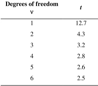
9.6. COMPLIANCE AGAINST LIMITS 30
APPENDIX A. EXAMPLES 32
INTRODUCTION 32
EXAMPLE A1: PREPARATION OF A CALIBRATION STANDARD 34
EXAMPLE A2: STANDARDISING A SODIUM HYDROXIDE SOLUTION 40
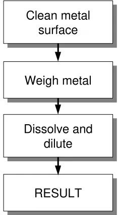
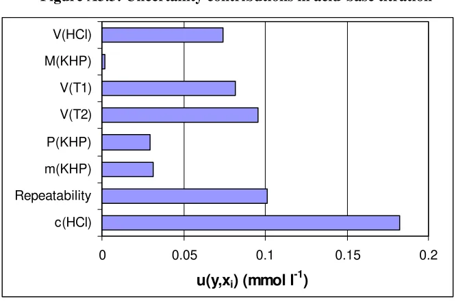
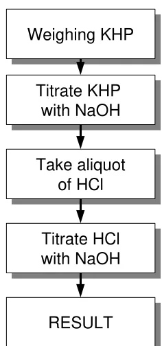
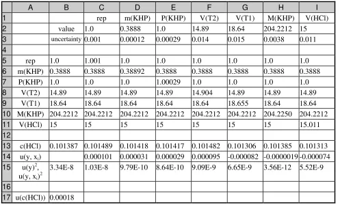
EXAMPLE A3: AN ACID/BASE TITRATION 50
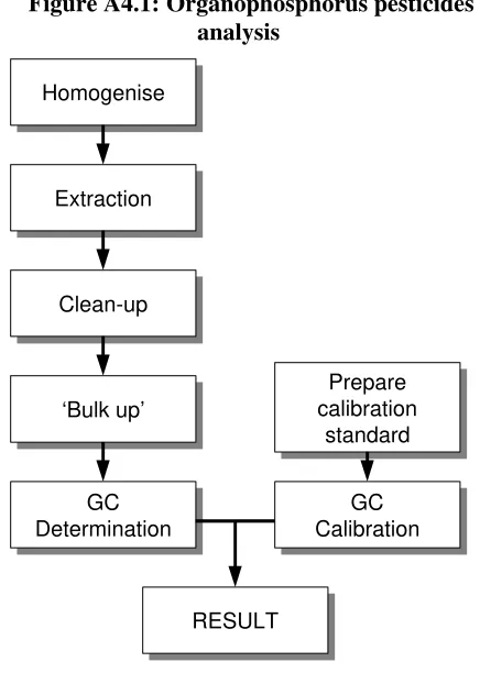
EXAMPLE A4: UNCERTAINTY ESTIMATION FROM IN-HOUSE VALIDATION STUDIES.
DETERMINATION OF ORGANOPHOSPHORUS PESTICIDES IN BREAD. 59
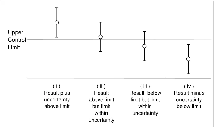
EXAMPLE A5: DETERMINATION OF CADMIUM RELEASE FROM CERAMIC WARE BY
ATOMIC ABSORPTION SPECTROMETRY 70
EXAMPLE A6: THE DETERMINATION OF CRUDE FIBRE IN ANIMAL FEEDING STUFFS 79
EXAMPLE A7: DETERMINATION OF THE AMOUNT OF LEAD IN WATER USING DOUBLE
ISOTOPE DILUTION AND INDUCTIVELY COUPLED PLASMA MASS SPECTROMETRY 87
APPENDIX B. DEFINITIONS 95
APPENDIX C. UNCERTAINTIES IN ANALYTICAL PROCESSES 99
APPENDIX D. ANALYSING UNCERTAINTY SOURCES 100
D.1 INTRODUCTION 100
D.2 PRINCIPLES OF APPROACH 100
D.3 CAUSE AND EFFECT ANALYSIS 100
D.4 EXAMPLE 101
APPENDIX E. USEFUL STATISTICAL PROCEDURES 102
E.1 DISTRIBUTION FUNCTIONS 102
E.2 SPREADSHEET METHOD FOR UNCERTAINTY CALCULATION 104 E.3 UNCERTAINTIES FROM LINEAR LEAST SQUARES CALIBRATION 106 E.4: DOCUMENTING UNCERTAINTY DEPENDENT ON ANALYTE LEVEL 108
APPENDIX F. MEASUREMENT UNCERTAINTY AT THE LIMIT OF DETECTION/
LIMIT OF DETERMINATION 112
F1. INTRODUCTION 112
F2. OBSERVATIONS AND ESTIMATES 112
F3. INTERPRETED RESULTS AND COMPLIANCE STATEMENTS 113
APPENDIX G. COMMON SOURCES AND VALUES OF UNCERTAINTY 114
Quantifying Uncertainty
Foreword to the Second Edition
Many important decisions are based on the results of chemical quantitative analysis; the results are used, for example, to estimate yields, to check materials against specifications or statutory limits, or to estimate monetary value. Whenever decisions are based on analytical results, it is important to have some indication of the quality of the results, that is, the extent to which they can be relied on for the purpose in hand. Users of the results of chemical analysis, particularly in those areas concerned with international trade, are coming under increasing pressure to eliminate the replication of effort frequently expended in obtaining them. Confidence in data obtained outside the user’s own organisation is a prerequisite to meeting this objective. In some sectors of analytical chemistry it is now a formal (frequently legislative) requirement for laboratories to introduce quality assurance measures to ensure that they are capable of and are providing data of the required quality. Such measures include: the use of validated methods of analysis; the use of defined internal quality control procedures; participation in proficiency testing schemes; accreditation based on ISO 17025 [H.1], and establishing traceabilityof the results of the measurements
In analytical chemistry, there has been great emphasis on the precision of results obtained using a specified method, rather than on their traceability to a defined standard or SI unit. This has led the use of “official methods” to fulfil legislative and trading requirements. However as there is now a formal requirement to establish the confidence of results it is essential that a measurement result is traceable to a defined reference such as a SI unit, reference material or, where applicable, a defined or empirical(sec. 5.2.) method. Internal quality control procedures, proficiency testing and accreditation can be an aid in establishing evidence of traceability to a given standard.
As a consequence of these requirements, chemists are, for their part, coming under increasing pressure to demonstrate the quality of their results, and in particular to demonstrate their fitness for purpose by giving a measure of the confidence that can be placed on the result. This is expected to include the degree to which a result would be expected to agree with other results, normally irrespective of the analytical methods used. One useful measure of this is measurement uncertainty.
Although the concept of measurement uncertainty has been recognised by chemists for many years, it was the publication in 1993 of the “Guide to the Expression of Uncertainty in Measurement” [H.2] by ISO in collaboration with BIPM, IEC, IFCC, IUPAC, IUPAP and OIML, which formally established general rules for evaluating and expressing uncertainty in measurement across a broad spectrum of measurements. This EURACHEM document shows how the concepts in the ISO Guide may be applied in chemical measurement. It first introduces the concept of uncertainty and the distinction between uncertainty and error. This is followed by a description of the steps involved in the evaluation of uncertainty with the processes illustrated by worked examples in Appendix A.
The evaluation of uncertainty requires the analyst to look closely at all the possible sources of uncertainty. However, although a detailed study of this kind may require a considerable effort, it is essential that the effort expended should not be disproportionate. In practice a preliminary study will quickly identify the most significant sources of uncertainty and, as the examples show, the value obtained for the combined uncertainty is almost entirely controlled by the major contributions. A good estimate of uncertainty can be made by concentrating effort on the largest contributions. Further, once evaluated for a given method applied in a particular laboratory (i.e. a particular measurement procedure), the uncertainty estimate obtained may be reliably applied to subsequent results obtained by the method in the same laboratory, provided that this is justified by the relevant quality control data. No further effort should be necessary unless the procedure itself or the equipment used is changed, in which case the uncertainty estimate would be reviewed as part of the normal re-validation.
Quantifying Uncertainty
Foreword to the Second Edition
This second edition of the EURACHEM Guide has been prepared in the light of practical experience of uncertainty estimation in chemistry laboratories and the even greater awareness of the need to introduce formal quality assurance procedures by laboratories. The second edition stresses that the procedures introduced by a laboratory to estimate its measurement uncertainty should be integrated with existing quality assurance measures, since these measures frequently provide much of the information required to evaluate the measurement uncertainty. The guide therefore provides explicitly for the use of validation and related data in the construction of uncertainty estimates in full compliance with formal ISO Guide principles. The approach is also consistent with the requirements of ISO 17025:1999 [H.1]
Quantifying Uncertainty
Scope and Field of Application
1.
Scope and Field of Application
1.1. This Guide gives detailed guidance for the evaluation and expression of uncertainty in quantitative chemical analysis, based on the approach taken in the ISO “Guide to the Expression of Uncertainty in Measurement” [H.2]. It is applicable at all levels of accuracy and in all fields - from routine analysis to basic research and to empirical and rational methods (see section 5.3.). Some common areas in which chemical measurements are needed, and in which the principles of this Guide may be applied, are:
• Quality control and quality assurance in manufacturing industries.
• Testing for regulatory compliance.
• Testing utilising an agreed method.
• Calibration of standards and equipment.
• Measurements associated with the development and certification of reference materials.
• Research and development.
1.2. Note that additional guidance will be required in some cases. In particular, reference material value assignment using consensus methods (including multiple measurement methods) is not covered, and the use of uncertainty estimates in compliance statements and the expression and use of uncertainty at low levels may require additional guidance. Uncertainties associated with sampling operations are not explicitly treated.
1.3. Since formal quality assurance measures have been introduced by laboratories in a number of sectors this second EURACHEM Guide is now able to illustrate how data from the following procedures may be used for the estimation of measurement uncertainty:
• Evaluation of the effect of the identified sources of uncertainty on the analytical result for a single method implemented as a defined measurementprocedure[B.8] in a single laboratory .
• Results from defined internal quality control procedures in a single laboratory.
• Results from collaborative trials used to validate methods of analysis in a number of competent laboratories.
• Results from proficiency test schemes used to assess the analytical competency of laboratories.
1.4. It is assumed throughout this Guide that, whether carrying out measurements or assessing the performance of the measurement procedure, effective quality assurance and control measures are in place to ensure that the measurement process is stable and in control. Such measures normally include, for example, appropriately qualified staff, proper maintenance and calibration of equipment and reagents, use of appropriate reference standards, documented measurement procedures and use of appropriate check standards and control charts. Reference [H.6] provides further information on analytical QA procedures. NOTE: This paragraph implies that all analytical methods are assumed in this guide to be implemented via fully
Quantifying Uncertainty
Uncertainty
2. Uncertainty
2.1. Definition of uncertainty
2.1.1. The definition of the term uncertainty (of measurement) used in this protocol and taken from the current version adopted for the International Vocabulary of Basic and General Terms in Metrology [H.4] is:
“A parameter associated with the result of a measurement, that characterises the dispersion of the values that could reasonably be attributed to the measurand”
Note 1 The parameter may be, for example, a
standard deviation [B.23] (or a given
multiple of it), or the width of a confidence interval.
NOTE 2 Uncertainty of measurement comprises, in general, many components. Some of these components may be evaluated from the statistical distribution of the results of series of measurements and can be characterised by standard deviations. The other components, which also can be characterised by standard deviations, are evaluated from assumed probability distributions based on experience or other information. The ISO Guide refers to these different cases as Type A and Type B estimations respectively.
2.1.2. In many cases in chemical analysis, the
measurand[B.6] will be the concentration* of an
analyte. However chemical analysis is used to measure other quantities, e.g. colour, pH, etc., and therefore the general term "measurand" will be used.
2.1.3. The definition of uncertainty given above focuses on the range of values that the analyst believes could reasonably be attributed to the measurand.
2.1.4. In general use, the word uncertainty relates to the general concept of doubt. In this guide, the
* In this guide, the unqualified term “concentration”
applies to any of the particular quantities mass concentration, amount concentration, number concentration or volume concentration unless units are quoted (e.g. a concentration quoted in mg l-1 is evidently a mass concentration). Note also that many other quantities used to express composition, such as mass fraction, substance content and mole fraction, can be directly related to concentration.
word uncertainty, without adjectives, refers either to a parameter associated with the definition above, or to the limited knowledge about a particular value. Uncertainty of measurement does not imply doubt about the validity of a measurement; on the contrary, knowledge of the uncertainty implies increased confidence in the validity of a measurement result.
2.2. Uncertainty sources
2.2.1. In practice the uncertainty on the result may arise from many possible sources, including examples such as incomplete definition, sampling, matrix effects and interferences, environmental conditions, uncertainties of masses and volumetric equipment, reference values, approximations and assumptions incorporated in the measurement method and procedure, and random variation (a fuller description of uncertainty sources is given in section 6.7.)
2.3. Uncertainty components
2.3.1. In estimating the overall uncertainty, it may be necessary to take each source of uncertainty and treat it separately to obtain the contribution from that source. Each of the separate contributions to uncertainty is referred to as an uncertainty component. When expressed as a standard deviation, an uncertainty component is known as a standard uncertainty [B.13]. If there is correlation between any components then this has to be taken into account by determining the covariance. However, it is often possible to evaluate the combined effect of several components. This may reduce the overall effort involved and, where components whose contribution is evaluated together are correlated, there may be no additional need to take account of the correlation.
2.3.2. For a measurement result y, the total
Quantifying Uncertainty
Uncertainty
2.3.3. For most purposes in analytical chemistry,
an expanded uncertainty [B.15] U, should be
used. The expanded uncertainty provides an interval within which the value of the measurand is believed to lie with a higher level of confidence. U is obtained by multiplying uc(y), the combined standard uncertainty, by a coverage factor [B.16] k. The choice of the factor k is based on the level of confidence desired. For an approximate level of confidence of 95%, k is 2.
NOTE The coverage factor k should always be stated so that the combined standard uncertainty of the measured quantity can be recovered for use in calculating the combined standard uncertainty of other measurement results that may depend on that quantity.
2.4. Error and uncertainty
2.4.1. It is important to distinguish between error and uncertainty. Error [B.19] is defined as the difference between an individual result and the
true value [B.3] of the measurand. As such,
error is a single value. In principle, the value of a known error can be applied as a correction to the result.
NOTE Error is an idealised concept and errors cannot be known exactly.
2.4.2. Uncertainty, on the other hand, takes the form of a range, and, if estimated for an analytical procedure and defined sample type, may apply to all determinations so described. In general, the value of the uncertainty cannot be used to correct a measurement result.
2.4.3. To illustrate further the difference, the result of an analysis after correction may by chance be very close to the value of the measurand, and hence have a negligible error. However, the uncertainty may still be very large, simply because the analyst is very unsure of how close that result is to the value.
2.4.4. The uncertainty of the result of a
measurement should never be interpreted as representing the error itself, nor the error remaining after correction.
2.4.5. An error is regarded as having two
components, namely, a random component and a systematiccomponent.
2.4.6. Random error [B.20] typically arises from unpredictable variations of influence quantities. These random effects give rise to variations in
repeated observations of the measurand. The random error of an analytical result cannot be compensated for, but it can usually be reduced by increasing the number of observations.
NOTE 1 The experimental standard deviation of the
arithmetic mean[B.22] or average of a series of observations is not the random error of the mean, although it is so referred to in some publications on uncertainty. It is instead a measure of the uncertainty of the mean due to some random effects. The exact value of the random error in the mean arising from these effects cannot be known.
2.4.7. Systematic error [B.21] is defined as a
component of error which, in the course of a number of analyses of the same measurand, remains constant or varies in a predictable way. It is independent of the number of measurements made and cannot therefore be reduced by increasing the number of analyses under constant measurement conditions.
2.4.8. Constant systematic errors, such as failing to make an allowance for a reagent blank in an assay, or inaccuracies in a multi-point instrument calibration, are constant for a given level of the measurement value but may vary with the level of the measurement value.
2.4.9. Effects which change systematically in
magnitude during a series of analyses, caused, for example by inadequate control of experimental conditions, give rise to systematic errors that are not constant.
EXAMPLES:
1. A gradual increase in the temperature of a set of samples during a chemical analysis can lead to progressive changes in the result.
2. Sensors and probes that exhibit ageing effects over the time-scale of an experiment can also introduce non-constant systematic errors.
2.4.10. The result of a measurement should be
corrected for all recognised significant systematic effects.
NOTE Measuring instruments and systems are often
adjusted or calibrated using measurement standards and reference materials to correct for systematic effects. The uncertainties associated with these standards and materials and the uncertainty in the correction must still be taken into account.
Quantifying Uncertainty
Uncertainty
failure or instrument malfunction. Transposing digits in a number while recording data, an air bubble lodged in a spectrophotometer flow-through cell, or accidental cross-contamination of test items are common examples of this type of error.
2.4.12. Measurements for which errors such as
these have been detected should be rejected and no attempt should be made to incorporate the errors into any statistical analysis. However, errors such as digit transposition can be corrected (exactly), particularly if they occur in the leading digits.
2.4.13. Spurious errors are not always obvious
and, where a sufficient number of replicate measurements is available, it is usually appropriate to apply an outlier test to check for the presence of suspect members in the data set. Any positive result obtained from such a test should be considered with care and, where possible, referred back to the originator for confirmation. It is generally not wise to reject a value on purely statistical grounds.
Quantifying Uncertainty
Analytical Measurement and Uncertainty
3. Analytical Measurement and Uncertainty
3.1. Method validation
3.1.1. In practice, the fitness for purpose of
analytical methods applied for routine testing is most commonly assessed through method validation studies [H.7]. Such studies produce data on overall performance and on individual influence factors which can be applied to the estimation of uncertainty associated with the results of the method in normal use.
3.1.2. Method validation studies rely on the
determination of overall method performance parameters. These are obtained during method development and interlaboratory study or following in-house validation protocols. Individual sources of error or uncertainty are typically investigated only when significant compared to the overall precision measures in use. The emphasis is primarily on identifying and removing (rather than correcting for) significant effects. This leads to a situation in which the majority of potentially significant influence factors have been identified, checked for significance compared to overall precision, and shown to be negligible. Under these circumstances, the data available to analysts consists primarily of overall performance figures, together with evidence of insignificance of most effects and some measurements of any remaining significant effects.
3.1.3. Validation studies for quantitative
analytical methods typically determine some or all of the following parameters:
Precision. The principal precision measures include repeatability standard deviation sr, reproducibility standard deviation sR, (ISO 3534-1) and intermediate precision, sometimes denoted sZi, with i denoting the number of factors varied (ISO 5725-3:1994). The repeatability sr indicates the variability observed within a laboratory, over a short time, using a single operator, item of equipment etc. sr may be estimated within a laboratory or by inter-laboratory study. Interlaboratory reproducibility standard deviation sR for a particular method may only be estimated directly by interlaboratory study; it shows the variability obtained when different laboratories analyse the same sample. Intermediate precision relates to the variation in results observed when
one or more factors, such as time, equipment and operator, are varied within a laboratory; different figures are obtained depending on which factors are held constant. Intermediate precision estimates are most commonly determined within laboratories but may also be determined by interlaboratory study. The observed precision of an analytical procedure is an essential component of overall uncertainty, whether determined by combination of individual variances or by study of the complete method in operation.
Bias. The bias of an analytical method is usually determined by study of relevant reference materials or by spiking studies. The determination of overall bias with respect to appropriate reference values is important in establishing
traceability [B.12] to recognised standards (see section 3.2). Bias may be expressed as analytical recovery (value observed divided by value expected). Bias should be shown to be negligible or corrected for, but in either case the uncertainty associated with the determination of the bias remains an essential component of overall uncertainty.
Linearity. Linearity is an important property of methods used to make measurements at a range of concentrations. The linearity of the response to pure standards and to realistic samples may be determined. Linearity is not generally quantified, but is checked for by inspection or using significance tests for non-linearity. Significant non-linearity is usually corrected for by use of non-linear calibration functions or eliminated by choice of more restricted operating range. Any remaining deviations from linearity are normally sufficiently accounted for by overall precision estimates covering several concentrations, or within any uncertainties associated with calibration (Appendix E.3).
Quantifying Uncertainty
Analytical Measurement and Uncertainty
Robustness or ruggedness. Many method development or validation protocols require that sensitivity to particular parameters be investigated directly. This is usually done by a preliminary ‘ruggedness test’, in which the effect of one or more parameter changes is observed. If significant (compared to the precision of the ruggedness test) a more detailed study is carried out to measure the size of the effect, and a permitted operating interval chosen accordingly. Ruggedness test data can therefore provide information on the effect of important parameters. Selectivity/specificity. Though loosely defined, both terms relate to the degree to which a method responds uniquely to the required analyte. Typical selectivity studies investigate the effects of likely interferents, usually by adding the potential interferent to both blank and fortified samples and observing the response. The results are normally used to demonstrate that the practical effects are not significant. However, since the studies measure changes in response directly, it is possible to use the data to estimate the uncertainty associated with potential interferences, given knowledge of the range of interferent concentrations.
3.2. Conduct of experimental studies of
method performance
3.2.1. The detailed design and execution of
method validation and method performance studies is covered extensively elsewhere [H.7] and will not be repeated here. However, the main principles as they affect the relevance of a study applied to uncertainty estimation are pertinent and are considered below.
3.2.2. Representativeness is essential. That is, studies should, as far as possible, be conducted to provide a realistic survey of the number and range of effects operating during normal use of the method, as well as covering the concentration ranges and sample types within the scope of the method. Where a factor has been representatively varied during the course of a precision experiment, for example, the effects of that factor appear directly in the observed variance and need no additional study unless further method optimisation is desirable.
3.2.3. In this context, representative variation means that an influence parameter must take a distribution of values appropriate to the uncertainty in the parameter in question. For continuous parameters, this may be a permitted range or stated uncertainty; for discontinuous
factors such as sample matrix, this range corresponds to the variety of types permitted or encountered in normal use of the method. Note that representativeness extends not only to the range of values, but to their distribution.
3.2.4. In selecting factors for variation, it is important to ensure that the larger effects are varied where possible. For example, where day to day variation (perhaps arising from recalibration effects) is substantial compared to repeatability, two determinations on each of five days will provide a better estimate of intermediate precision than five determinations on each of two days. Ten single determinations on separate days will be better still, subject to sufficient control, though this will provide no additional information on within-day repeatability.
3.2.5. It is generally simpler to treat data obtained from random selection than from systematic variation. For example, experiments performed at random times over a sufficient period will usually include representative ambient temperature effects, while experiments performed systematically at 24-hour intervals may be subject to bias due to regular ambient temperature variation during the working day. The former experiment needs only evaluate the overall standard deviation; in the latter, systematic variation of ambient temperature is required, followed by adjustment to allow for the actual distribution of temperatures. Random variation is, however, less efficient. A small number of systematic studies can quickly establish the size of an effect, whereas it will typically take well over 30 determinations to establish an uncertainty contribution to better than about 20% relative accuracy. Where possible, therefore, it is often preferable to investigate small numbers of major effects systematically.
3.2.6. Where factors are known or suspected to
interact, it is important to ensure that the effect of interaction is accounted for. This may be achieved either by ensuring random selection from different levels of interacting parameters, or by careful systematic design to obtain both variance and covariance information.
3.2.7. In carrying out studies of overall bias, it is important that the reference materials and values are relevant to the materials under routine test.
3.2.8. Any study undertaken to investigate and
Quantifying Uncertainty
Analytical Measurement and Uncertainty
3.3. Traceability
3.3.1. It is important to be able to compare results from different laboratories, or from the same laboratory at different times, with confidence. This is achieved by ensuring that all laboratories are using the same measurement scale, or the same ‘reference points’. In many cases this is achieved by establishing a chain of calibrations leading to primary national or international standards, ideally (for long-term consistency) the Systeme Internationale (SI) units of measurement. A familiar example is the case of analytical balances; each balance is calibrated using reference masses which are themselves checked (ultimately) against national standards and so on to the primary reference kilogram. This unbroken chain of comparisons leading to a known reference value provides ‘traceability’ to a common reference point, ensuring that different operators are using the same units of measurement. In routine measurement, the consistency of measurements between one laboratory (or time) and another is greatly aided by establishing traceability for all relevant intermediate measurements used to obtain or control a measurement result. Traceability is therefore an important concept in all branches of measurement.
3.3.2. Traceability is formally defined [H.4]as: “The property of the result of a measurement or the value of a standard whereby it can be related to stated references, usually national or international standards, through an unbroken chain of comparisons all having stated uncertainties.”
The reference to uncertainty arises because the agreement between laboratories is limited, in part, by uncertainties incurred in each laboratory’s traceability chain. Traceability is accordingly intimately linked to uncertainty. Traceability provides the means of placing all related measurements on a consistent measurement scale, while uncertainty characterises the ‘strength’ of the links in the chain and the agreement to be expected between laboratories making similar measurements.
3.3.3. In general, the uncertainty on a result
which is traceable to a particular reference, will be the uncertainty on that reference together with the uncertainty on making the measurement relative to that reference.
3.3.4. Traceability of the result of the complete analytical procedure should be established by a combination of the following procedures:
1. Use of traceable standards to calibrate the measuring equipment
2. By using, or by comparison to the results of, a primary method
3. By using a pure substance RM.
4. By using an appropriate matrix Certified Reference Material (CRM)
5. By using an accepted, closely defined procedure.
Each procedure is discussed in turn below.
3.3.5. Calibration of measuring equipment
In all cases, the calibration of the measuring equipment used must be traceable to appropriate standards. The quantification stage of the analytical procedure is often calibrated using a pure substance reference material, whose value is traceable to the SI. This practice provides traceability of the results to SI for this part of the procedure. However, it is also necessary to establish traceability for the results of operations prior to the quantification stage, such as extraction and sample clean up, using additional procedures.
3.3.6. Measurements using Primary Methods
A primary method is currently described as follows:
“A primary method of measurement is a method having the highest metrological qualities, whose operation is completely described and understood in terms of SI units and whose results are accepted without reference to a standard of the same quantity.” The result of a primary method is normally traceable directly to the SI, and is of the smallest achievable uncertainty with respect to this reference. Primary methods are normally implemented only by National Measurement Institutes and are rarely applied to routine testing or calibration. Where applicable, traceability to the results of a primary method is achieved by direct comparison of measurement results between the primary method and test or calibration method.
3.3.7. Measurements using a pure substance Reference Material (RM).
Quantifying Uncertainty
Analytical Measurement and Uncertainty
containing, a known quantity of a pure substance RM. This may be achieved, for example, by spiking or by standard additions. However, it is always necessary to evaluate the difference in response of the measurement system to the standard used and the sample under test. Unfortunately, for many chemical analyses and in the particular case of spiking or standard additions, both the correction for the difference in response and its uncertainty may be large. Thus, although the traceability of the result to SI units can in principle be established, in practice, in all but the most simple cases, the uncertainty on the result may be unacceptably large or even unquantifiable. If the uncertainty is unquantifiable then traceability has not been established
3.3.8. Measurement on a Certified Reference Material (CRM)
Traceability may be demonstrated through comparison of measurement results on a certified matrix CRM with the certified value(s). This procedure can reduce the uncertainty compared to the use of a pure substance RM where there is a suitable matrix CRM available. If the value of the CRM is traceable to SI, then these measurements provide traceability to SI units and the evaluation of the uncertainty utilising
reference materials is discussed in 7.5. However, even in this case, the uncertainty on the result may be unacceptably large or even unquantifiable, particularly if there is not a good match between the composition of the sample and the reference material.
3.3.9. Measurement using an accepted procedure.
Quantifying Uncertainty
The Uncertainty Estimation Process
4. The Process of Measurement Uncertainty Estimation
4.1. Uncertainty estimation is simple in principle. The following paragraphs summarise the tasks that need to be performed in order to obtain an estimate of the uncertainty associated with a measurement result. Subsequent chapters provide additional guidance applicable in different circumstances, particularly relating to the use of data from method validation studies and the use of formal uncertainty propagation principles. The steps involved are:
Step 1. Specify measurand
Write down a clear statement of what is being measured, including the relationship between the measurand and the input quantities (e.g. measured quantities, constants, calibration standard values etc.) upon which it depends. Where possible, include corrections for known systematic effects. The specification information should be given in the relevant Standard Operating Procedure (SOP) or other method description.
Step 2. Identify uncertainty sources
List the possible sources of uncertainty. This will include sources that contribute to the uncertainty on the parameters in the relationship specified in Step 1, but may include other sources and must include sources arising from chemical assumptions. A general procedure for forming a structured list is suggested at Appendix D.
Step 3. Quantify uncertainty components
Measure or estimate the size of the uncertainty component associated with each potential source of uncertainty identified. It is often possible to estimate or determine a single contribution to uncertainty associated with a number of separate sources. It is also important to consider whether available data accounts sufficiently for all sources of uncertainty, and plan additional experiments and studies carefully to ensure that all sources of uncertainty are adequately accounted for.
Step 4. Calculate combined uncertainty
The information obtained in step 3 will consist of a number of quantified contributions to overall uncertainty, whether associated with individual sources or with the combined effects of several sources. The contributions have to be expressed as standard deviations, and combined according to the appropriate rules, to give a combined standard uncertainty. The appropriate coverage factor should be applied to give an expanded uncertainty.
Figure 1 shows the process schematically.
4.2. The following chapters provide guidance
Quantifying Uncertainty
The Uncertainty Estimation Process
Figure 1: The Uncertainty Estimation Process
Specify Measurand
Identify Uncertainty
Sources
Simplify by grouping sources
covered by existing data
Quantify remaining components
Quantify grouped components
Convert components to standard deviations
Calculate combined standard uncertainty
END
Calculate Expanded uncertainty Review and if necessary re-evaluate
large components START
Step 1
Step 2
Step 3
Quantifying Uncertainty
Step 1. Specification of the Measurand
5.
Step 1. Specification of the Measurand
5.1. In the context of uncertainty estimation, “specification of the measurand” requires both a clear and unambiguous statement of what is being measured, and a quantitative expression relating the value of the measurand to the parameters on which it depends. These parameters may be other measurands, quantities which are not directly measured, or constants. It should also be clear whether a sampling step is included within the procedure or not. If it is, estimation of uncertainties associated with the sampling procedure need to be considered. All of this information should be in the Standard Operating Procedure (SOP).
5.2. In analytical measurement, it is particularly important to distinguish between measurements intended to produce results which are independent of the method used, and those which are not so intended. The latter are often referred to as empirical methods. The following examples may clarify the point further.
EXAMPLES:
1. Methods for the determination of the amount of nickel present in an alloy are normally expected to yield the same result, in the same units, usually expressed as a mass or mole fraction. In principle, any systematic effect due to method bias or matrix would need to be corrected for, though it is more usual to ensure that any such effect is small. Results would not normally need to quote the particular method used, except for information. The method is not empirical.
2. Determinations of “extractable fat” may differ substantially, depending on the extraction
conditions specified. Since “extractable fat” is entirely dependent on choice of conditions, the method used is empirical. It is not meaningful to consider correction for bias intrinsic to the method, since the measurand is defined by the method used. Results are generally reported with reference to the method, uncorrected for any bias intrinsic to the method. The method is considered empirical.
3. In circumstances where variations in the substrate, or matrix, have large and unpredictable effects, a procedure is often developed with the sole aim of achieving comparability between laboratories measuring the same material. The procedure may then be adopted as a local, national or international standard method on which trading or other decisions are taken, with no intent to obtain an absolute measure of the true amount of analyte present. Corrections for method bias or matrix effect are ignored by convention (whether or not they have been minimised in method development). Results are normally reported uncorrected for matrix or method bias. The method is considered to be empirical.
Quantifying Uncertainty
6.
Step 2. Identifying Uncertainty Sources
6.1. A comprehensive list of relevant sources of uncertainty should be assembled. At this stage, it is not necessary to be concerned about the quantification of individual components; the aim is to be completely clear about what should be considered. In Step 3, the best way of treating each source will be considered.
6.2. In forming the required list of uncertainty sources it is usually convenient to start with the basic expression used to calculate the measurand from intermediate values. All the parameters in this expression may have an uncertainty associated with their value and are therefore potential uncertainty sources. In addition there may be other parameters that do not appear explicitly in the expression used to calculate the value of the measurand, but which nevertheless affect the measurement results, e.g. extraction time or temperature. These are also potential sources of uncertainty. All these different sources should be included. Additional information is given in Appendix C (Uncertainties in Analytical Processes).
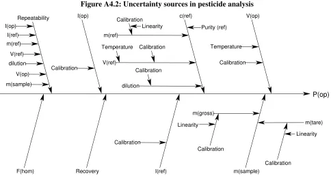
6.3. The cause and effect diagram described in
Appendix D is a very convenient way of listing the uncertainty sources, showing how they relate to each other and indicating their influence on the uncertainty of the result. It also helps to avoid double counting of sources. Although the list of uncertainty sources can be prepared in other ways, the cause and effect diagram is used in the following chapters and in all of the examples in Appendix A. Additional information is given in Appendix D (Analysing uncertainty sources).
6.4. Once the list of uncertainty sources is
assembled, their effects on the result can, in principle, be represented by a formal measurement model, in which each effect is associated with a parameter or variable in an equation. The equation then forms a complete model of the measurement process in terms of all the individual factors affecting the result. This function may be very complicated and it may not be possible to write it down explicitly. Where possible, however, this should be done, as the form of the expression will generally determine the method of combining individual uncertainty contributions.
6.5. It may additionally be useful to consider a measurement procedure as a series of discrete operations (sometimes termed unit operations), each of which may be assessed separately to obtain estimates of uncertainty associated with them. This is a particularly useful approach where similar measurement procedures share common unit operations. The separate uncertainties for each operation then form contributions to the overall uncertainty.
6.6. In practice, it is more usual in analytical measurement to consider uncertainties associated with elements of overall method performance, such as observable precision and bias measured with respect to appropriate reference materials. These contributions generally form the dominant contributions to the uncertainty estimate, and are best modelled as separate effects on the result. It is then necessary to evaluate other possible contributions only to check their significance, quantifying only those that are significant. Further guidance on this approach, which applies particularly to the use of method validation data, is given in section 7.2.1.
6.7. Typical sources of uncertainty are
• Sampling
Where in-house or field sampling form part of the specified procedure, effects such as random variations between different samples and any potential for bias in the sampling procedure form components of uncertainty affecting the final result.
• Storage Conditions
Where test items are stored for any period prior to analysis, the storage conditions may affect the results. The duration of storage as well as conditions during storage should therefore be considered as uncertainty sources.
• Instrument effects
Quantifying Uncertainty
Step 2. Identifying Uncertainty Sources
differs (within specification) from its indicated set-point; an auto-analyser that could be subject to carry-over effects.
• Reagent purity
The concentration of a volumetric solution will not be known exactly even if the parent material has been assayed, since some uncertainty related to the assaying procedure remains. Many organic dyestuffs, for instance, are not 100% pure and can contain
isomers and inorganic salts. The purity of such substances is usually stated by manufacturers as being not less than a specified level. Any assumptions about the degree of purity will introduce an element of uncertainty.
• Assumed stoichiometry
Where an analytical process is assumed to follow a particular reaction stoichiometry, it may be necessary to allow for departures from the expected stoichiometry, or for incomplete reaction or side reactions.
• Measurement conditions
For example, volumetric glassware may be used at an ambient temperature different from that at which it was calibrated. Gross temperature effects should be corrected for, but any uncertainty in the temperature of liquid and glass should be considered. Similarly, humidity may be important where materials are sensitive to possible changes in humidity.
• Sample effects
The recovery of an analyte from a complex matrix, or an instrument response, may be affected by composition of the matrix. Analyte speciation may further compound this effect.
The stability of a sample/analyte may change during analysis because of a changing thermal regime or photolytic effect.
When a ‘spike’ is used to estimate recovery, the recovery of the analyte from the sample may differ from the recovery of the spike, introducing an uncertainty which needs to be evaluated.
• Computational effects
Selection of the calibration model, e.g. using a straight line calibration on a curved response, leads to poorer fit and higher uncertainty.
Truncation and round off can lead to inaccuracies in the final result. Since these are rarely predictable, an uncertainty allowance may be necessary.
• Blank Correction
There will be an uncertainty on both the value and the appropriateness of the blank correction. This is particularly important in trace analysis.
• Operator effects
Possibility of reading a meter or scale consistently high or low.
Possibility of making a slightly different interpretation of the method.
• Random effects
Random effects contribute to the uncertainty in all determinations. This entry should be included in the list as a matter of course.
Quantifying Uncertainty
Step 3. Quantifying Uncertainty
7. Step 3. Quantifying Uncertainty
7.1. Introduction
7.1.1. Having identified the uncertainty sources as explained in Step 2 (Chapter 6), the next step is to quantify the uncertainty arising from these sources. This can be done by
• evaluating the uncertainty arising from each individual source and then combining them as described in Chapter 8. Examples A1 to A3 illustrate the use of this procedure.
or
• by determining directly the combined contribution to the uncertainty on the result from some or all of these sources using method performance data. Examples A4 to A6 represent applications of this procedure. In practice, a combination of these is usually necessary and convenient.
7.1.2. Whichever of these approaches is used,
most of the information needed to evaluate the uncertainty is likely to be already available from the results of validation studies, from QA/QC data and from other experimental work that has been carried out to check the performance of the method. However, data may not be available to evaluate the uncertainty from all of the sources and it may be necessary to carry out further work as described in sections 7.10. to 7.14.
7.2. Uncertainty evaluation procedure
7.2.1. The procedure used for estimating the
overall uncertainty depends on the data available about the method performance. The stages involved in developing the procedure are
• Reconcile the information requirements
with the available data
First, the list of uncertainty sources should be examined to see which sources of uncertainty are accounted for by the available data, whether by explicit study of the particular contribution or by implicit variation within the course of whole-method experiments. These sources should be checked against the list prepared in Step 2 and any remaining sources should be listed to provide an auditable record of which contributions to the uncertainty have been included.
• Plan to obtain the further data required
For sources of uncertainty not adequately covered by existing data, either seek additional information from the literature or standing data (certificates, equipment specifications etc.), or plan experiments to obtain the required additional data. Additional experiments may take the form of specific studies of a single contribution to uncertainty, or the usual method performance studies conducted to ensure representative variation of important factors.
7.2.2. It is important to recognise that not all of the components will make a significant contribution to the combined uncertainty; indeed, in practice it is likely that only a small number will. Unless there is a large number of them, components that are less than one third of the largest need not be evaluated in detail. A preliminary estimate of the contribution of each component or combination of components to the uncertainty should be made and those that are not significant eliminated.
Quantifying Uncertainty
Step 3. Quantifying Uncertainty
7.3. Relevance of prior studies
7.3.1. When uncertainty estimates are based at
least partly on prior studies of method performance, it is necessary to demonstrate the validity of applying prior study results. Typically, this will consist of:
• Demonstration that a comparable precision to that obtained previously can be achieved.
• Demonstration that the use of the bias data obtained previously is justified, typically through determination of bias on relevant reference materials (see, for example, ISO Guide 33 [H.8]), by appropriate spiking studies, or by satisfactory performance on relevant proficiency schemes or other laboratory intercomparisons.
• Continued performance within statistical control as shown by regular QC sample results and the implementation of effective analytical quality assurance procedures.
7.3.2. Where the conditions above are met, and
the method is operated within its scope and field of application, it is normally acceptable to apply the data from prior studies (including validation studies) directly to uncertainty estimates in the laboratory in question.
7.4. Evaluating uncertainty by
quantification of individual
components
7.4.1. In some cases, particularly when little or no method performance data is available, the most suitable procedure may be to evaluate each uncertainty component separately.
7.4.2. The general procedure used in combining
individual components is to prepare a detailed quantitative model of the experimental procedure (cf. sections 5. and 6., especially 6.4.), assess the standard uncertainties associated with the individual input parameters, and combine them using the law of propagation of uncertainties as described in Section 8.
7.4.3. In the interests of clarity, detailed guidance on the assessment of individual contributions by experimental and other means is deferred to sections 7.10. to 7.14. Examples A1 to A3 in Appendix A provide detailed illustrations of the procedure. Extensive guidance on the application of this procedure is also given in the ISO Guide [H.2].
7.5. Closely matched certified
reference materials
7.5.1. Measurements on certified reference
materials are normally carried out as part of method validation or re-validation, effectively constituting a calibration of the whole measurement procedure against a traceable reference. Because this procedure provides information on the combined effect of many of the potential sources of uncertainty, it provides very good data for the assessment of uncertainty. Further details are given in section 7.7.4. NOTE: ISO Guide 33 [H.8] gives a useful account of
the use of reference materials in checking method performance.
7.6. Uncertainty estimation using prior
collaborative method development
and validation study data
7.6.1. A collaborative study carried out to
validate a published method, for example according to the AOAC/IUPAC protocol [H.9] or ISO 5725 standard [H.10], is a valuable source of data to support an uncertainty estimate. The data typically include estimates of reproducibility standard deviation, sR, for several levels of response, a linear estimate of the dependence of sR on level of response, and may include an estimate of bias based on CRM studies. How this data can be utilised depends on the factors taken into account when the study was carried out. During the ‘reconciliation’ stage indicated above (section 7.2.), it is necessary to identify any sources of uncertainty that are not covered by the collaborative study data. The sources which may need particular consideration are:
• Sampling. Collaborative studies rarely include a sampling step. If the method used in-house involves sub-sampling, or the measurand (see Specification) is estimating a bulk property from a small sample, then the effects of sampling should be investigated and their effects included.
• Pre-treatment. In most studies, samples are homogenised, and may additionally be stabilised, before distribution. It may be necessary to investigate and add the effects of the particular pre-treatment procedures applied in-house.
Quantifying Uncertainty
Step 3. Quantifying Uncertainty
methods or materials. Where the bias itself, the uncertainty in the reference values used, and the precision associated with the bias check, are all small compared to sR, no additional allowance need be made for bias uncertainty. Otherwise, it will be necessary to make additional allowances.
• Variation in conditions.
Laboratories participating in a study may tend towards the means of allowed ranges of experimental conditions, resulting in an underestimate of the range of results possible within the method definition. Where such effects have been investigated and shown to be insignificant across their full permitted range, however, no further allowance is required.
• Changes in sample matrix. The uncertainty arising from matrix compositions or levels of interferents outside the range covered by the study will need to be considered.
7.6.2. Each significant source of uncertainty not covered by the collaborative study datashould be evaluated in the form of a standard uncertainty and combined with the reproducibility standard deviation sR in the usual way (section 8.)
7.6.3. For methods operating within their defined scope, when the reconciliation stage shows that all the identified sources have been included in the validation study or when the contributions from any remaining sources such as those discussed in section 7.6.1. have been shown to be negligible, then the reproducibility standard deviation sR, adjusted for concentration if necessary, may be used as the combined standard uncertainty.
7.6.4. The use of this procedure is shown in
example A6 (Appendix A)
7.7. Uncertainty estimation using
in-house development and validation
studies
7.7.1. In-house development and validation
studies consist chiefly of the determination of the method performance parameters indicated in section 3.1.3. Uncertainty estimation from these parameters utilises:
• The best available estimate of overall precision.
• The best available estimate(s) of overall bias and its uncertainty.
• Quantification of any uncertainties associated with effects incompletely accounted for in the above overall performance studies.
Precision study
7.7.2. The precision should be estimated as far as possible over an extended time period, and chosen to allow natural variation of all factors affecting the result. This can be obtained from
• The standard deviation of results for a typical sample analysed several times over a period of time, using different analysts and equipment where possible (the results of measurements on QC check samples can provide this information).
• The standard deviation obtained from replicate analyses performed on each of several samples.
NOTE: Replicates should be performed at materially different times to obtain estimates of intermediate precision; within-batch replication provides estimates of repeatability only.
• From formal multi-factor experimental designs, analysed by ANOVA to provide separate variance estimates for each factor.
7.7.3. Note that precision frequently varies
significantly with the level of response. For example, the observed standard deviation often increases significantly and systematically with analyte concentration. In such cases, the uncertainty estimate should be adjusted to allow for the precision applicable to the particular result. Appendix E.4 gives additional guidance on handling level-dependent contributions to uncertainty.
Bias study
7.7.4. Overall bias is best estimated by repeated analysis of a relevant CRM, using the complete measurement procedure. Where this is done, and the bias found to be insignificant, the uncertainty associated with the bias is simply the combination of the standard uncertainty on the CRM value with the standard deviation associated with the bias.
NOTE: Bias estimated in this way combines bias in laboratory performance with any bias intrinsic to the method in use. Special considerations may apply where the method in use is empirical; see section 7.8.1.
Quantifying Uncertainty
Step 3. Quantifying Uncertainty
materials, additional factors should be considered, including (as appropriate) differences in composition and homogeneity; reference materials are frequently more homogeneous that test samples. Estimates based on professional judgement should be used, if necessary, to assign these uncertainties (see section 7.14.).
• Any effects following from different concentrations of analyte; for example, it is not uncommon to find that extraction losses differ between high and low levels of analyte.
7.7.5. Bias for a method under study can also be determined by comparison of the results with those of a reference method. If the results show that the bias is not statistically significant, the standard uncertainty is that for the reference method (if applicable; see section 7.8.1.), combined with the standard uncertainty associated with the measured difference between methods. The latter contribution to uncertainty is given by the standard deviation term used in the significance test applied to decide whether the difference is statistically significant, as explained in the example below.
EXAMPLE
A method (method 1) for determining the concentration of Selenium is compared with a reference method (method 2). The results (in mg kg-1) from each method are as follows:
x s n
Method 1 5.40 1.47 5 Method 2 4.76 2.75 5 The standard deviations are pooled to give a pooled standard deviation sc
205 . 2 2 5 5 ) 1 5 ( 75 . 2 ) 1 5 ( 47 .
1 2 2
= − + − × + − × = c s
and a corresponding value of t:
46 . 0 4 . 1 64 . 0 5 1 5 1 205 . 2 ) 76 . 4 40 . 5 ( = = + − = t
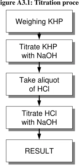
tcrit is 2.3 for 8 degrees of freedom, so there is no significant difference between the means of the results given by the two methods. However, the difference (0.64) is compared with a standard deviation term of 1.4 above. This value of 1.4 is the standard deviation associated with the difference, and accordingly represents the relevant contribution to uncertainty associated with the measured bias.
7.7.6. Overall bias can also be estimated by the addition of analyte to a previously studied material. The same considerations apply as for the study of reference materials (above). In addition, the differential behaviour of added material and material native to the sample should be considered and due allowance made. Such an allowance can be made on the basis of:
• Studies of the distribution of the bias observed for a range of matrices and levels of added analyte.
• Comparison of result observed in a reference material with the recovery of added analyte in the same reference material.
• Judgement on the basis of specific materials with known extreme behaviour. For example, oyster tissue, a common marine tissue reference, is well known for a tendency to co-precipitate some elements with calcium salts on digestion, and may provide an estimate of ‘worst case’ recovery on which an uncertainty estimate can be based (e.g. By treating the worst case as an extreme of a rectangular or triangular distribution).
• Judgement on the basis of prior experience.
7.7.7. Bias may also be estimated by comparison of the particular method with a value determined by the method of standard additions, in which known quantities of the analyte are added to the test material, and the correct analyte concentration inferred by extrapolation. The uncertainty associated with the bias is then normally dominated by the uncertainties associated with the extrapolation, combined (where appropriate) with any significant contributions from the preparation and addition of stock solution.
NOTE: To be directly relevant, the additions should be made to the original sample, rather than a prepared extract.
7.7.8. It is a general requirement of the ISO Guide that corrections should be applied for all recognised and significant systematic effects. Where a correction is applied to allow for a significant overall bias, the uncertainty associated with the bias is estimated as paragraph 7.7.5. described in the case of insignificant bias
7.7.9. Where the bias is significant, but is
Quantifying Uncertainty
Step 3. Quantifying Uncertainty
Additional factors
7.7.10. The effects of any remaining factors
should be estimated separately, either by experimental variation or by prediction from established theory. The uncertainty associated with such factors should be estimated, recorded and combined with other contributions in the normal way.
7.7.11. Where the effect of these remaining
factors is demonstrated to be negligible compared to the precision of the study (i.e. statistically insignificant), it is recommended that an uncertainty contribution equal to the standard deviation associated with the relevant significance test be associated with that factor. EXAMPLE
The effect of a permitted 1-hour extraction time variation is investigated by a t-test on five determinations each on the same sample, for the normal extraction time and a time reduced by 1 hour. The means and standard deviations (in mg l-1) were: Standard time: mean 1.8, standard deviation 0.21; alternate time: mean 1.7, standard deviation 0.17. A t-test uses the pooled variance of 037 . 0 ) 1 5 ( ) 1 5 ( 17 . 0 ) 1 5 ( 21 . 0 ) 1 5
( 2 2
= − + − × − + × − to obtain 82 . 0 5 1 5 1 037 . 0 ) 7 . 1 8 . 1 ( = + × − = t
This is not significant compared to tcrit = 2.3. But note that the difference (0.1) is compared with a calculated standard deviation term of
) 5 / 1 5 / 1 ( 037 .
0 × + =0.12. This value is the contribution to uncertainty associated with the effect of permitted variation in extraction time.
7.7.12. Where an effect is detected and is
statistically significant, but remains sufficiently small to neglect in practice, the provisions of section 7.15. apply.
7.8. Evaluation of uncertainty for
empirical methods
7.8.1.An ‘empirical method’ is a method agreed
upon for the purposes of comparative measurement within a particular field of application where the measurand characteristically depends upon the method in use. The method accordingly defines the measurand. Examples include methods for
leachable metals in ceramics and dietary fibre in foodstuffs (see also section 5.2. and example A5)
7.8.2. Where such a method is in use within its defined field of application, the bias associated with the method is defined as zero. In such circumstances, bias estimation need relate only to the laboratory performance and should not additionally account for bias intrinsic to the method. This has the following implications.
7.8.3. Reference material investigations, whether to demonstrate negligible bias or to measure bias, should be conducted using reference materials certified using the particular method, or for which a value obtained with the particular method is available for comparison.
7.8.4. Where reference materials so characterised are unavailable, overall control of bias is associated with the control of method parameters affecting the result; typically such factors as times, temperatures, masses, volumes etc. The uncertainty associated with these input factors must accordingly be assessed and either shown to be negligible or quantified (see example A6).
7.8.5. Empirical methods are normally subjected to collaborative studies and hence the uncertainty can be evaluated as described in section 7.6.
7.9. Evaluation of uncertainty for
ad-hoc methods
7.9.1. Ad-hoc methods are methods established to carry out exploratory studies in the short term, or for a short run of test materials. Such methods are typically based on standard or well-established methods within the laboratory, but are adapted substantially (for example to study a different analyte) and will not generally justify formal validation studies for the particular material in question.
Quantifying Uncertainty
Step 3. Quantifying Uncertainty
the uncertainty in these blocks has been established previously.
7.9.3. As a minimum, it is essential that an
estimate of overall bias and an indication of precision be available for the method in question. Bias will ideally be measured against a reference material, but will in practice more commonly be assessed from spike recovery. The considerations of section 7.7.4. then apply, except that spike recoveries should be compared with those observed on the related system to establish the relevance of the prior studies to the ad-hoc method in question. The overall bias observed for the ad-hoc method, on the materials under test, should be comparable to that observed for the related system, within the requirements of the study.
7.9.4. A minimum precision experiment consists
of a duplicate analysis. It is, however, recommended that as many replicates as practical are performed. The precision should be compared with that for the related system; the standard deviation for the ad-hoc method should be comparable.
NOTE: It recommended that the comparison be based on inspection. Statistical significance tests (e.g. an F-test) will generally be unreliable with small numbers of replicates and will tend to lead to the conclusion that there is ‘no significant difference’ simply because of the low power of the test.
7.9.5. Where the above conditions are met
unequivocally, the uncertainty estimate for the related system may be applied directly to results obtained by the ad-hoc method, making any adjustments appropriate for concentration dependence and other known factors.
7.10. Quantification of individual
components
7.10.1. It is nearly always necessary to consider some sources of uncertainty individually. In some cases, this is only necessary for a small number of sources; in others, particularly when little or no method performance data is available, every source may need separate study (see examples 1,2 and 3 in Appendix A for illustrations). There are several general methods for establishing individual uncertainty components:
§ Experimental variation of input variables
§ From standing data such as measurement and calibration certificates
§ By modelling from theoretical principles
§ Using judgement based on experience or informed by modelling of assumptions These different methods are discussed briefly below.
7.11. Experimental estimation of
individual uncertainty
contributions
7.11.1. It is often possible and practical to obtain estimates of uncertainty contributions from experimental studies specific to individual parameters.
7.11.2. The standard uncertainty arising from
random effects is often measured from repeatability experiments and is quantified in terms of the standard deviation of the measured values. In practice, no more than about fifteen replicates need normally be considered, unless a high precision is required.
7.11.3. Other typical experiments include:
• Study of the effect of a variation of a single parameter on the result. This is particularly appropriate in the case of continuous, controllable parameters, independent of other effects, such as time or temperature. The rate of change of the result with the change in the parameter can be obtained from the experimental data. This is then combined directly with the uncertainty in the parameter to obtain the relevant uncer