Estimation of the Reproductive Number and the Serial Interval in
Early Phase of the 2009 Influenza the Current Influenza A/H1N1
Pandemic in the USA
Laura Forsberg White*
Department of Biostatistics 801 Massachusetts Ave Boston University School of Public Health Boston, MA, USA 02118
Jacco Wallinga
Centre for Infectious Disease Control Netherlands National Institute of Public Health and the Environment Bilthoven, Netherlands
Julius Center for Health Sciences and Primary Care University Medical Center Utrecht, Utrecht, Netherlands
Lyn Finelli and Carrie Reed
Epidemiology and Prevention Branch, Influenza Division NCIRD, CDC Atlanta GA, USA
Steven Riley
School of Public Health and Department of Community Medicine The University of Hong Kong
Marc Lipsitch
Department of Epidemiology Harvard School of Public Health Boston, MA, USA
Marcello Pagano
Department of Biostatistics Harvard School of Public Health Boston, MA, USA
Abstract
Background—The United States was the second country to have a major outbreak of novel influenza A/H1N1 in what has become a new pandemic. Appropriate public health responses to this pandemic depend in part on early estimates of key epidemiological parameters of the virus in defined populations.
Methods—We use a likelihood-based method to estimate the basic reproductive number (R0)
and serial interval using individual level US data from the Centers for Disease Control and Prevention (CDC). We adjust for missing dates of illness and changes in case ascertainment. Using prior estimates for the serial interval we also estimate the reproductive number only.
Results—Using the raw CDC data, we estimate the reproductive number to be between 2.2 and 2.3 and the mean of the serial interval (μ) between 2.5 and 2.6 days. After adjustment for
increased case ascertainment our estimates change to 1.7 to 1.8 for R0 and 2.2 to 2.3 days for μ. In
a sensitivity analysis making use of previous estimates of the mean of the serial interval, both for this epidemic (μ =1.91 days) and for seasonal influenza (μ =3.6 days), we estimate the
reproductive number at 1.5 to 3.1.
Conclusions—With adjustments for data imperfections we obtain useful estimates of key epidemiological parameters for the current Influenza H1N1 outbreak in the United States. Estimates that adjust for suspected increases in reporting suggest that substantial reductions in the
NIH Public Access
Author Manuscript
Influenza Other Respi Viruses. Author manuscript; available in PMC 2010 November 1.
Published in final edited form as:
Influenza Other Respi Viruses. 2009 November ; 3(6): 267–276. doi:10.1111/j.1750-2659.2009.00106.x.
NIH-PA Author Manuscript
NIH-PA Author Manuscript
spread of this epidemic may be achievable with aggressive control measures, while sensitivity analyses suggest the possibility that even such measures would have limited effect in reducing total attack rates.
Keywords
Influenza A/H1N1 Outbreak; basic reproductive number; serial interval
Introduction
In April 2009 the general public became aware of an outbreak of a novel influenza strain, now termed novel Influenza A/H1N1 that had been affecting Mexico. Due to high travel volumes throughout the world, particularly the United States, the disease has been spreading rapidly worldwide, and in May 2009 led the WHO to raise the pandemic alert to a level 5, indicating that a pandemic is likely imminent and signaling world health organizations and governments to finalize planning and preparation for responding to such an event. On June 11 WHO declared a pandemic had begun.
While most cases have been relatively mild outside of Mexico (1), a number of uncertainties remain about the severity of this virus on a per-case basis; moreover, higher-than-normal attack rates expected from an antigenically novel virus may lead to substantial population-level severe morbidity and mortality even if the case-fatality ratio remains low (2).
Regardless of the severity now, legitimate concerns exist over the potential impact that this viral strain might have in the coming influenza season. Indeed during the high mortality pandemic of 1918–1919, much of the northern hemisphere saw a mild outbreak in the late spring of 1918 that preceded the much more severe outbreaks of the fall and winter of 1918– 1919(3,4). For these reasons, continuing scientific and public health attention to the spread of this novel virus is essential.
As officials prepare and plan for the growth of this pandemic, estimates of epidemiological parameters are needed to mount an effective response. Decisions about the degree of mitigation that is warranted – and public compliance with efforts to reduce transmission – depend in part on estimates of individual and population risk, as measured in part by the frequency of severe and fatal illness. Knowledge of the serial interval and basic reproductive number are crucial for understanding the dynamics of any infectious disease, and these should be reevaluated as the pandemic progresses in space and time (5). The basic reproductive number R0 is defined as the average number of secondary cases per typical
case in an otherwise susceptible population, and is a special case of the more general reproductive number, which may be measured even after some of the population is immune. R0 quantifies the transmissibility of an infection: the higher the R0, the more difficult it is to
control. The distribution of the serial interval, the time between infections in consecutive generations, determines, along with R0, the rate at which an epidemic grows. Estimates of
these quantities characterize the rates of epidemic growth and informs recommendations for control measures; ongoing estimates of the reproductive number as control measures are introduced can be used to estimate the impact of control measures. Previous modeling work has stated that a reproductive number exceeding two for influenza would make it unlikely that even stringent control measures could halt the growth of an influenza pandemic (6).
Prior work has placed estimates for the serial interval of seasonal influenza at 3.6 days (7) with a standard deviation of 1.6 days. Other work has estimated that the serial interval is between 2.8 and 3.3 days (8). Analysis of linked cases of novel A/H1N1 in Spain yields an estimate of a mean of 3.5 days with a range from one to six days (9). Fraser et al (10) estimate the mean of the serial interval to be 1.91 days for the completed outbreak of
NIH-PA Author Manuscript
NIH-PA Author Manuscript
respiratory infection in La Gloria, Mexico, which may have resulted from the novel H1N1 strain. There have been many attempts made to estimate the reproductive number. Fraser et al (10) estimate the reproductive number to be in the range of 1.4–1.6 for La Gloria but acknowledge the preliminary nature of their estimate. For the fall wave of the 1918 pandemic, others have estimated the basic reproductive number to be approximately 1.8 for UK cities (11), 2.0 for US cities (12), 1.34–3.21 (depending on the setting) (8) and 1.2–1.5 (3). Additionally Viboud et al. (3) estimate, in contrast, that the reproductive number in the 1918 summer wave was between 2.0 and 5.4.
In what follows we employ a likelihood based method previously introduced (8,13) to simultaneously estimate the basic reproductive number and the serial interval. We make use of data from the Centers for Disease Control (CDC) providing information on all early reported cases in the United States, including the date of symptom onset and report. Further, we illustrate the impact of the reporting fraction and temporal trends in the reporting fraction on estimates of these parameters.
Methods
Data
We use data from the Centers for Disease Control and Prevention (CDC) line list of reported cases of Influenza A/H1N1 in the United States beginning on March 28, 2009. Information about 1368 confirmed and probable cases with a date of report on or before May 8, 2009 was used. Of the 1368 reported cases, 750 had a date of onset recorded. We include probable cases in the analysis as >90% of probable cases subsequently tested have been confirmed. After May 13 collection of individual-based data became much less frequent and eventually halted in favor of aggregate counts of new cases. The degree of case ascertainment early throughout this time period is unknown.
Statistical Analysis
We make use of the likelihood based method of White and Pagano (8,13). This method is well-suited for estimation of the basic reproductive number, R0, and the serial interval in
real time with observed aggregated daily counts of new cases, denoted by N={N0, N1, …,
NT} where T is the last day of observation and N0 are the initial number of seed cases that
begin the outbreak. The Ni are assumed to be composed of a mixture of cases that were
generated by the previous k days, where k is the maximal value of the serial interval. We denote these as Xji, the number of cases that appear on day i that were infected by
individuals with onset of symptoms on day j. We assume that the number of infectees
generated by infectors with symptoms on day j, , follows a Poisson
distribution with parameter R0Nj. Additionally, Xj = {Xj,j+1, Xj,j+2,…,Xj,j+k+1}, the vector of cases infected by the Nj individuals, follows a multinomial distribution with parameters p, k
and Xj. here p is a vector of probabilities thet denotes the serial interval distrisbuttion. Using
these assumptions, we obtain the fllowing likelihood, as shown in white and pagano (13):
where and Γ(x) is the gamma function. Maximizing the likelihood over
R0 and p provides estimators for the reproductive number and serial interval. This method
assumes that there are no imported cases, there is no missing data and that the population is
NIH-PA Author Manuscript
NIH-PA Author Manuscript
uniformly mixing. Assuming that there are imported cases (for example individuals who became infected in Mexico after the index case), denoted by Y = {Y1,…YT, then the likelihood becomes
where φt, is defined as before.
We further modify this methodology to account for some of the imperfections of the current data.
Imputation of missing onset times—First, we handle missing onset times by making use of the reporting delay distribution. Most cases have a date of report, but far fewer have a date of onset given. As our interest is in modeling the date of onset, we impute these missing dates for those with a date of report. Let rti be the reporting time, let oti be their time of
onset, assuming it is observed, and let dti= rti− oti. We fit a linear regression model with the
log(dti) as the outcome and rti as the explanatory variable as well as an indicator of whether
the case is an imported case or not, bti. For each person with a reported rti but missing oti, we
obtain oti by predicting the value for the reporting delay from the model, denoted by
, and generate a random variable Xti, as the exponential of a normally distributed
random variable with parameter and variance given by the prediction error
from the regression model. Then the imputed time of onset is: , where [Xti] is the rounded value. The data used in this analysis is , where Nt is the number of observed onset times for day t and are the number of unobserved (and thus imputed) onset times on day t.
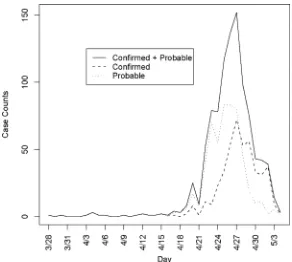
Augmentation of data for underreporting—As observed in Figure 1, the onset times are rapidly declining as one approaches the final date of report. This is likely attributable to reporting lag and is addressed by inflating case counts to account for delayed reporting. Again using the reporting delay distribution, we can modify the number of cases with onset
on day t, as , where qj is the probability of a j day reporting delay and l
is the length of the reporting delay distribution. Note that the Mt are often non integer values
since they are estimates of the true number of cases. We only consider Mt such that the
augmented data represents no more than 95% of the imputed reported value.
Adjustment for changes in reporting fraction—Further, we report on the impact of changes in reporting. Inevitably many cases will go undetected. It is reasonable to assume that the proportion that go undetected will initially decrease as an epidemic unfolds and the public becomes increasingly aware of the outbreak. It is estimated that during the
exponential growth phase of the epidemic, the proportion of hospitalized persons among cases reported between April 13 and April 28, declined at a rate of 10% per day (data not shown). We interpret this as an increase in the rate of ascertainment, i.e. the average severity of infections was not decreasing. Rather, the proportion of cases being ascertained was increasing with more mild cases being ascertained. Therefore, we estimate that the ratio of observed cases on consecutive days was 90% of the ratio of the true number of cases during this time. If st of the true cases are reported on day t and Nt cases are observed on that day,
then
NIH-PA Author Manuscript
NIH-PA Author Manuscript
.
This implies that st =(1/0.9)st-1 will be reported on day t, representing a 11% increase in
reporting with time. In the analysis, we modify the likelihood by inflating expected counts by 1/s,s={s1,…,sT} per day, but do not take account of the binomial variation in reported
cases that is associated with less than perfect reporting. We assume that st=0.15 for t=1,…,
15 (i.e. March 28 to April 13) and thereafter st=1.11 st-1. We report on sensitivity to these
assumptions.
Spectral analysis of the cyclical component of the epidemic curve—As an independent check of our joint estimation of R0 and the serial interval, we used an
alternative method to estimate the serial interval from the observed epidemiological curve. The idea is that we decompose the observed epidemiological curve into a trend component, which is essentially a moving average over d days, and a cyclical component, which is the difference between the observed number of cases and the trend. We expect that if there are a few cases in excess over the trend at day t, these cases will result in secondary cases that form an excess over the trend near day t + μ, and tertiary cases that form an excess over the trend near day t + 2μ and so on. Therefore we expect to see positive autocorrelation in the cyclical component of the epidemiological curve with a characteristic period equal to the mean of the serial interval μ. The characteristic period can be extracted using spectral analysis. Here we used the spectrum() command with modified Daniell smoothers as encoded in the R package. We expect the characteristic period of μ days to show up as a dominant frequency of (1/μ) (day−1).
Interquartile ranges for the estimates were obtained by using a parametric bootstrap. 1000 simulated datasets were generated using the parameter estimates and constrained to have a total epidemic size within 2% of the actual epidemic size. The 0.025 and 0.975 quantiles obtained from the simulated data are reported as the confidence interval. All analyses were performed using R 2.6.1.
Results
The data are shown in Figure 1 by date of onset. There were 1368 confirmed or probable cases with a recorded date of report. Of these, there were 750 with a recorded date of onset. The first date of onset is March 28, 2009. The last date of onset is May 4, 2009 making 38 days of data used in the analysis. Over this period of time 117 of the reported cases had recently traveled to Mexico and are considered imported cases in our analysis. We report results for four separate data sets: all data with an onset date on or before April 25, 26, 27 or 29. Further, by the end of April knowledge of the epidemic was widespread in the US and reporting mechanisms began to change, such that cases began to be reported in batches and were less likely to include individual information on the date of onset.
Estimation of R0 and the Serial Interval
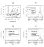
Reporting delays by day of onset for cases with known date of onset are shown in Fig. 2(a) The results from the regression indicate that a reporting date that is one day later is associated with a 5% increase in the reporting delay (p<0.001).
NIH-PA Author Manuscript
NIH-PA Author Manuscript
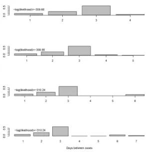
We first show the results from imputing and then augmenting the data to obtain and Mt in Figure 2. Our initial interest is in determining the optimal value for k (the maximum serial interval category) to be used in the analysis. We allow k to vary between four and seven days and obtain the estimates for the serial interval using data with onset times on or before the 27th day of the epidemic (April 24, 2009). In interpreting the serial interval curves in Figure 3, it should be noted that the final category represents the probability of a serial interval of k days or longer. On the basis of these results, we set k to four since the log likelihood values for the varying values of k are nearly indistinguishable and in all cases the major mass (on average 88% for the original data and 93% for the augmented data) of the serial interval lies in the first three days.
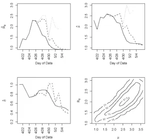
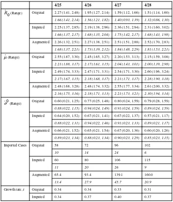
We obtain estimates using the original data (Nt), the imputed data ( ) and the augmented data (Mt) shown in Table 1 and Figure 4. Clearly using all available data will lead to biased results since significant underreporting is occurring from April 29 onward when the epidemic curve begins to plummet. In Figure 4 we show results using data with onset dates up to and including each day from April 21, 2009 through May 4, 2009. The reliability of the results using the actual data is questionable since so many issues in the data have not been accounted for. Augmenting and imputing the data appears to stabilize the estimates substantially. We further note in the final pane of Figure 4 the dependence between the estimates. Using data from simulated outbreaks, we estimate the bivariate density of the basic reproductive number and the mean of the serial interval using a bivariate kernel density estimator. Not surprisingly this illustrates the positive correlation between the basic reproductive number and the mean of the serial interval.
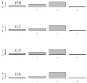
Using the observed data when the peak number of incident cases is observed, we obtain the serial interval estimates shown in Figure 5. The estimated mean of the serial interval tends to be between 2.5 and 2.6 days for all the data, with a mode of three days. R0 is estimated to be
between 2.3 and 2.5 for data ending between April 25 and April 27. We observe growth rates, r, between 0.34 and 0.43, depending on the data used (Table 1).
Additionally, we observe that when we account for increases in the reporting fraction, the
estimates of the reproductive number drop substantially and the estimates of
the mean serial interval decrease by about 10% (2.2–2.3 days, see Table 1). We note the sensitivity of these estimates to the assumed reporting distribution and report these sensitivities for estimates obtained on April 27 using the imputed data where and
. Given a reporting fraction increase of 11%/day, if the initial reporting fraction varies between s0=0.01 and s0=0.20 then will range between 1.91 (s0 =0.01) and 1.71 (s0
=0.20) and the estimated mean serial interval will vary between 2.19 (s0 =0.01) and 2.22 (s0 =0.20). If the daily rate of change in the reporting ratio varies from 11% to values between 8% and 14% and we hold s0 =0.15, then a ranges between 1.98 (8%) and 1.63 (14%) and
is estimated to be between 2.28 (8%) and 2.16 (14%).
Finally, we assess the trend component of the epidemiological curve using a moving average over d=4 days, and we assess the cyclical component as the deviation between the observed number of cases and the trend. We only use data up to April 28, 2009. For the original data we find a dominant frequency of 0.4, suggesting a serial interval of 2.5 days. Repeating this with the imputed data suggests a serial interval of 2.67 days, and the augmented data suggests a serial interval of 3.2 days. These results are similar to the findings on the modal serial interval (3 days) from maximum likelihood estimation, though slightly higher than the estimated mean serial interval. This suggests that the estimated values for serial intervals are
NIH-PA Author Manuscript
NIH-PA Author Manuscript
based on regularities in deviations from the trend in the epidemiological curve. There were no indications of weekly periodicity or a weekday effect.
Estimation of R0 alone
Estimates for the serial interval in a different setting have recently been provided by Cowling et al (7) and Fraser et al (10). The first is for seasonal influenza and obtained using household transmission data. The authors fit the observed serial interval estimates to a Weibull distribution with a mean of 3.6 days and standard deviation of 1.6 days. This estimate is consistent with that obtained by the Spanish surveillance group (9) for the current Influenza A/H1N1 outbreak. Fraser et al (10) estimate the mean of the serial interval to be 1.91 days for the present virus in La Gloria, Mexico. While both serial interval and reproductive number are likely to depend on the virus and also on the population, we consider a sensitivity analysis in which we assume previously measured serial interval distributions and estimate the reproductive number alone (Table 2). To use the Fraser et al estimate, we assume that the standard deviation is one day and that the serial interval follows a discretized gamma distribution. We also use a discretized gamma distribution while preserving the mean and standard deviation of the Cowling et al estimate (7). In both cases we set k to 6.
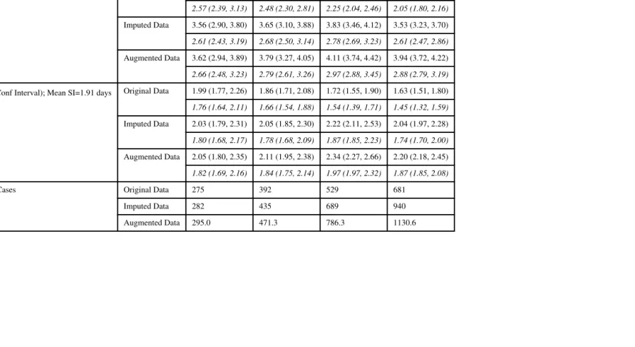
Our results are as expected and indicate that the estimated reproductive number varies dramatically depending on the estimate of the serial interval used. For the longer estimate of Cowling et al, the estimates ranged between 3.25 and 4.67 using the observed data. For the serial interval estimate derived from Fraser et al, the estimates are much lower, and are between 1.92 and 2.52.
The italicized entries in Table 2 provides estimates of the reproductive number under the same circumstances as previously stated but also taking into account the possibility that reporting increased by 11.1% each day starting April 13. Unsurprisingly, estimates decline under this assumption. For the Fraser et al serial interval, the estimated reproductive number falls to between 1.5 and 2.0, whereas for the Cowling et al estimate the value is between 2.0 and 3.0.
These estimates were similarly sensitive to assumptions on the initial reporting fraction and its rate of change starting April 13. For values of the initial reporting fraction from 0.01 to 0.20 for the imputed data on April 27, then the estimate of R0 will range between 3.03 and 2.70 for the Cowling serial interval and 2.03 and 1.81 for the Fraser serial interval. Varying the daily rate of change in the reporting fraction from 8% to 14% rather than being fixed at 11% than the estimates would range between 3.19 and 2.54 for the Cowling estimate and 2.06 and 1.75 for the Fraser estimate. The larger the initial reporting fraction or the larger the increase in the reporting ratio, the greater proportion of cases that are reported throughout the time of observation. This increase in reporting leads to a decrease in the estimate of the reproductive number.
Discussion
We obtain estimates of the reproductive number and the serial interval. These estimates, along with information on population susceptibility and risk of severe disease, help to inform public health policy, such as potential utility or success of different community mitigation strategies, and help to characterize the spread of the disease. Our estimates of the early reproductive number of novel influenza A/H1N1 in the United States are higher than those obtained in another published study of data from the Netherlands (14) and Mexico (10). Our estimates are slightly smaller than those obtained from an initial analysis of the outbreak in Japan (15) and an alternative analysis of data from Mexico (16). There are
NIH-PA Author Manuscript
NIH-PA Author Manuscript
several possible explanations for this. First, the prior estimates were based on a completed outbreakof a respiratory infection in La Gloria, Mexico and on virus genetic data, whereas our study uses the early phase of the epidemic curve from the United States as a whole. Each of these data sets has various uncertainties associated with it; we have highlighted and attempted to correct for changes in reporting, reporting delays, and missing dates of onset, but these corrections will only be approximate. Indeed, all data sets for an infection with a spectrum of severity and changing ascertainment patterns will be imperfect in these ways. Second, we have used a different approach (8,13) from that used in the Mexico data; results reported here use a method focused on a period of exponential growth of the epidemic, while the prior estimates used either viral sequence coalescence estimates or analysis of a whole epidemic curve, including the declining phase, in the case of La Gloria. Finally, our estimate of the serial interval from the data is longer than that obtained for La Gloria, though somewhat shorter than that obtained from contact tracing in Spain (9). As expected, if we assume a serial interval distribution, rather than estimate it, our estimate of the reproductive number shifts to adjust, as a consequence of the relationship between these two quantities (17,18).
The results presented here should be interpreted with the following caveats in mind. First the data is not from a closed system, and clearly there are imported cases, such as individuals who acquired the illness in Mexico after March 28. Although we account for cases that are known to be imported, it is likely that the data we have is incomplete and several other infections could have been imported. Misclassification of cases that were truly imported will bias reproductive number estimates upwards. Second, incomplete reporting is a feature of nearly all data on the novel influenza A/H1N1, and certainly of any data sets large enough to estimate temporal trends in case numbers. If underreporting were consistent over time, it would have only a minor effect on our point estimates (which depend mainly on the growth rate and on cyclical signals in the data) but would increase uncertainty around these estimates. More likely, as we have noted, there are trends in reporting, with increasing reporting as awareness grows, and declining reporting as public health workers become unable to obtain and report detailed information on each case. One might argue for analyzing only a subset of cases during the time period with optimal reporting or by only looking at hospitalizations, which might be more accurately recorded. However, in the first case, we ignore a large number of initial cases that will undoubtedly lead to gross errors in the estimates. In this case all secondary cases after the first day that is analyzed will be attributable to that day. By only considering hospitalizations, we violate the assumption of a closed system and assume that all cases that are hospitalized are attributable to another hospitalized case. The results from such an analysis would be challenging to interpret. Instead, we have accounted for these changes by imputation of onset dates, augmentation of data to account for reporting delays, and adjustments for an estimated upward trend in reporting of the early data. We feel that such adjustments, while still imperfect, are superior to ignoring information in incomplete data. In all analyses of such data, the statistical confidence intervals obtained should not be interpreted as measuring all of the uncertainty in estimates; additional uncertainty comes from unmeasured changes in reporting.
We have also noted the impact of the assumed reporting distribution on the estimates with a sensitivity analysis. While we have estimated the rate of increase in the reporting fraction through time from our data, our estimate of the initial reporting fraction is not based on data. We have illustrated the impact of variation in these quantities on our estimates and note that while our estimates do change as these quantities vary the changes are not dramatic. In fact if we assume that the initial reporting fraction is as low as 1% rather than our assumed 15%, then the estimate of the reproductive number increases from 1.75 to 1.90. The impact that the difference in these two estimates will have on policy is minimal. We also note that under the same circumstances, the estimated mean of the serial interval changes very little (from
NIH-PA Author Manuscript
NIH-PA Author Manuscript
2.21 to 2.19), illustrating the robustness of the mean to variations in this quantity. What these results mean is that as fewer of the cases are reported, our estimates of the
reproductive number are likely to be overly conservative if we do not properly adjust for this underreporting.
We have discussed the impact of the assumed serial interval on the estimates of the reproductive number. It is clear that assuming a form of the serial interval directly impacts the estimates of the reproductive number. External estimates of the serial interval
distribution have the advantage that they are directly observed rather than inferred from properties of the epidemic curve; on the other hand, pairs of cases with known infector and infectee are nonrepresentative of the overall pattern of transmission in a population. For our baseline results, we estimate the serial interval nonparametrically rather than imposing a shape on it. We have also incorporated previous estimates of serial interval to test the sensitivity of our conclusions.
The difference between our low estimates (when assuming increased reporting fraction and using Fraser et al. (10)'s serial interval distribution from La Gloria) and our high estimates (when ignoring increased reporting and using the serial interval distribution of Cowling et al. for seasonal influenza(7)) is the difference between an epidemic that is readily controlled and one that is virtually uncontrollable according to existing models of pandemic
interventions (6,11,19). It is clear that more precise estimates of the serial interval in various contexts for this virus are essential to reduce the uncertainty of estimates of the reproductive number; similarly, it is essential to estimate growth rates in a variety of contexts where reporting fractions can be better understood, possibly at local levels where a single reporting system is used.
Finally, it should be remembered that neither serial interval (20,21) nor reproductive number is a constant of nature; each depends on the population, the state of control measures and behavior, and other factors. Continued monitoring of the growth of the pandemic in various settings will be required to define the range of reproductive numbers achieved by this virus and their possible dependence on geography, population, season, and changes in the virus.
Acknowledgments
This work was funded in part by the National Institutes of Health, R01 EB0061695 and Models of Infectious Disease Agents Study program through cooperative agreements 5U01GM076497 and and 1U54GM088588 to ML, the latter for the Harvard Center for Communicable Disease Dynamics.
References
1. Novel Swine-Origin Influenza A (H1N1) Virus Investigation Team. Emergence of a novel swine-origin influenza A (H1N1) virus in humans. N Engl J Med. 2009:0.
2. Lipsitch M, Riley S, Cauchemez S, Ghani AC, Ferguson NM. Managing and reducing uncertainty in an emerging influenza pandemic. N Engl J Med. 2009; 0:1.
3. Andreasen V, Viboud C, Simonsen L. Epidemiologic characterization of the 1918 influenza pandemic summer wave in copenhagen: Implications for pandemic control strategies. J Infect Dis. Jan 15; 2008 197(2):270–8. [PubMed: 18194088]
4. Barry JM, Viboud C, Simonsen L. Cross-protection between successive waves of the 1918–1919 influenza pandemic: Epidemiological evidence from US army camps and from britain. J Infect Dis. Nov 15; 2008 198(10):1427–34. [PubMed: 18808337]
5. Fraser C, Riley S, Anderson RM, Ferguson NM. Factors that make an infectious disease outbreak controllable. Proc Natl Acad Sci U S A. Apr 20; 2004 101(16):6146–51. [PubMed: 15071187]
NIH-PA Author Manuscript
NIH-PA Author Manuscript
6. Halloran ME, Ferguson NM, Eubank S, Longini IM Jr, Cummings DA, Lewis B, et al. Modeling targeted layered containment of an influenza pandemic in the united states. Proc Natl Acad Sci U S A. Mar 25; 2008 105(12):4639–44. [PubMed: 18332436]
7. Cowling BJ, Fang VJ, Riley S, Malik Peiris JS, Leung GM. Estimation of the serial interval of influenza. Epidemiology. May; 2009 20(3):344–7. [PubMed: 19279492]
8. White LF, Pagano M. Transmissibility of the influenza virus in the 1918 pandemic. PLoS ONE. Jan 30.2008 3(1):e1498. [PubMed: 18231585]
9. Surveillance Group for New Influenza A(H1N1) Virus Investigation and Control in Spain. New influenza A(H1N1) virus infections in spain, april-may 2009. Eurosurveillance. 2009; 14(19) 10. Fraser C, Donnelly CA, Cauchemez S, Hanage WP, Van Kerkhove MD, Hollingsworth TD, et al.
Pandemic potential of a strain of influenza A (H1N1): Early findings. Science. May 14.2009 11. Ferguson NM, Cummings DA, Cauchemez S, Fraser C, Riley S, Meeyai A, et al. Strategies for
containing an emerging influenza pandemic in southeast asia. Nature. Sep 8; 2005 437(7056):209– 14. [PubMed: 16079797]
12. Mills CE, Robins JM, Lipsitch M. Transmissibility of 1918 pandemic influenza. Nature. Dec 16; 2004 432(7019):904–6. [PubMed: 15602562]
13. White LF, Pagano M. A likelihood-based method for real-time estimation of the serial interval and reproductive number of an epidemic. Stat Med. Jul 20; 2008 27(16):2999–3016. [PubMed: 18058829]
14. Hahne S, Donker T, Meijer A, Timen A, van Steenbergen J, Osterhaus A, et al. Epidemiology and control of influenza A(H1N1)v in the netherlands: The first 115 cases. Euro Surveill. Jul 9.2009 14(27):19267. [PubMed: 19589332]
15. Nishiura H, Castillo-Chavez C, Safan M, Chowell G. Transmission potential of the new influenza A(H1N1) virus and its age-specificity in japan. Euro Surveill. Jun 4.2009 14(22):19227. [PubMed: 19497256]
16. Boelle PY, Bernillon P, Desenclos JC. A preliminary estimation of the reproduction ratio for new influenza A(H1N1) from the outbreak in mexico, march–april 2009. Euro Surveill. May 14.2009 14(19):19205. [PubMed: 19442402]
17. Lipsitch M, Bergstrom CT. Invited commentary: Real-time tracking of control measures for emerging infections. Am J Epidemiol. Sep 15.2004 160(6):517, 9. discussion 520. [PubMed: 15353410]
18. Anderson, RM.; May, RM. Infectious diseases of humans. Oxford University Press; Oxford, U.K.: 1991.
19. Germann TC, Kadau K, Longini IM Jr, Macken CA. Mitigation strategies for pandemic influenza in the united states. Proc Natl Acad Sci U S A. Apr 11; 2006 103(15):5935–40. [PubMed: 16585506]
20. Kenah E, Lipsitch M, Robins JM. Generation interval contraction and epidemic data analysis. Math Biosci. May; 2008 213(1):71–9. [PubMed: 18394654]
21. Svensson A. A note on generation times in epidemic models. Math Biosci. Jul; 2007 208(1):300– 11. [PubMed: 17174352]
NIH-PA Author Manuscript
NIH-PA Author Manuscript
Figure 1.
Confirmed and probable cases in the United States plotted by onset time. First date of onset is March 28, 2009.
NIH-PA Author Manuscript
NIH-PA Author Manuscript
Figure 2.
(a) Reporting delay by the date of report. (b) Imputed data and original data, (c) All data(right frame), (d) only augmented data where at least 5% of the data is observed.
NIH-PA Author Manuscript
NIH-PA Author Manuscript
Figure 3.
Serial interval estimates for k=4, 5, 6, and 7 days with -log(likelihood) values.
NIH-PA Author Manuscript
NIH-PA Author Manuscript
Figure 4.
Estimates for the reproductive number, and mean and variance of th serial interval. The results using the original data (solid line), imputed data (dashed e line) and augmented data (dotted line) are all shown using data with onset date no later than the value in the x axis. Augmented data estimates are not shown after Ap correspond, in part to those shown in Table 1. The fourth pane shows the contour ril 30, 2009 since less than 5% of the data is original data. These results correspond, in part to those shown in Table 1. The fourth pane shows the contour plot of the joint density estimate of the mean of the serial interval and the basic reproductive number for imputed data up thto and including April 27. The values of the contours correspond the estimated 25th, 50th, 75th and 97.5th percentiles of the joint density.
NIH-PA Author Manuscript
NIH-PA Author Manuscript
Figure 5.
Serial interval estimate using data up to and including 4/25/2009 (top figure), 4/26/2009 (second), 4/27/2009 (third) and 4/28/2009 (bottom figure).
NIH-PA Author Manuscript
NIH-PA Author Manuscript
White et al.
Page 16
Table 1
Estimates obtained from the original, imputed and augmented data. Bootstrap confidence intervals are shown. Italicized results reflect results accounting for an 11% per day increase in reporting fraction starting April 13.
4/25 4/26 4/27 4/28
R^0 (Range) Original 2.27 (1.41, 2.48) 1.95 (1.27, 2.14) 1.59 (1.12, 1.66) 1.51 (1.14, 1.60) 1.66 (1.41, 2.14) 1.56 (1.21, 1.82) 1.40 (0.93, 1.39) 1.32 (0.86, 1.30)
Imputed 2.25 (1.37, 2.85) 2.19 (1.38, 2.96) 2.36 (1.51, 2.94) 2.31 (1.60, 3.02)
1.66 (1.37, 2.17) 1.68 (1.35, 2.04) 1.75 (1.42, 2.17) 1.68 (1.43, 1.98)
Augmented 2.26 (1.32, 2.51) 2.27 (1.38, 2.51) 2.51 (1.51, 2.88) 2.52 (1.70, 2.83)
1.68 (1.37, 2.21) 1.73 (1.39, 2.12) 1.84 (1.48, 2.29) 1.81 (1.53, 2.21)
μ^ (Range) Original 2.55 (1.87, 3.30) 2.45 (1.65, 3.27) 2.20 (1.53, 3.13) 2.15 (1.59, 3.08) 2.21 (1.88, 3.17) 2.17 (1.61, 3.15) 2.04 (1.43, 3.01) 2.00 (1.39, 2.98)
Imputed 2.49 (1.74, 3.33) 2.47 (1.71, 3.31) 2.54 (1.71, 3.30) 2.60 (1.96, 3.24)
2.17 (1.67, 3.15) 2.18 (1.68, 3.17) 2.21 (1.71, 3.17) 2.28 (1.90, 3.18)
Augmented 2.48 (1.68, 3.28) 2.48 (1.74, 3.32) 2.55 (1.77, 3.34) 2.61 (2.00, 3.32)
2.16 (1.75, 3.16) 2.18 (1.71, 3.13) 2.21 (1.73, 3.21) 2.30 (1.94, 3.14)
σ^0 (Range) Original 0.60 (0.21, 1.25) 0.77 (0.25, 1.48) 0.80 (0.24, 1.59) 0.79 (0.28, 1.59) 0.88 (0.22, 1.15) 0.94 (0.24, 1.49) 0.91 (0.24, 1.59) 0.89 (0.24, 1.59)
Imputed 0.64 (0.20, 1.52) 0.67 (0.21, 1.41) 0.67 (0.22, 1.37) 0.57 (0.21, 1.17)
0.88 (0.22, 1.31) 0.94 (0.22, 1.46) 0.91 (0.23, 1.33) 0.89 (0.21, 1.17)
Augmented 0.66 (0.21, 1.52) 0.65 (0.21, 1.54) 0.67 (0.20, 1.36) 0.60 (0.20, 1.26)
0.89 (0.23, 1.34) 0.88 (0.23, 1.34) 0.90 (0.23, 1.29) 0.85 (0.23, 1.15)
Imported Cases Original 58 72 96 102
10 14 24 6
Imputed 60 80 106 115
11 20 26 9
Augmented 65.4 93.4 139.1 160.0
13.4 27.9 45.7 20.9
Growth rate, r Original 0.34 0.34 0.33 0.31
Imputed 0.34 0.37 0.40 0.37
Influenza Other Respi Viruses
White et al.
Page 17
4/25 4/26 4/27 4/28
Augmented 0.35 0.39 0.43 0.41
New Cases Original 78 117 137 152
Imputed 85 153 254 251
Augmented 91.6 176.3 314.9 344.4
Total Cases Original 275 392 529 681
Imputed 282 435 689 940
Augmented 295.0 471.3 786.3 1130.6
Influenza Other Respi Viruses
White et al.
Page 18
Table 2
Estimates of the reproductive number the mean of the serial interval is 3.6 days with standard deviation of 1.6 days (7) or mean of 1.91 days and standard deviation of 1 days (10). Italicized results reflect results accounting for an 11% per day increase in reporting fraction starting April 13.
4/25/09 4/26/09 4/27/09 4/28/09
R^0 (Conf Interval); Mean SI=3.6 days Original Data 3.48 (2.88, 3.72) 3.29 (2.85, 3.47) 2.87 (2.55, 3.06) 2.59 (2.31, 2.77) 2.57 (2.39, 3.13) 2.48 (2.30, 2.81) 2.25 (2.04, 2.46) 2.05 (1.80, 2.16)
Imputed Data 3.56 (2.90, 3.80) 3.65 (3.10, 3.88) 3.83 (3.46, 4.12) 3.53 (3.23, 3.70)
2.61 (2.43, 3.19) 2.68 (2.50, 3.14) 2.78 (2.69, 3.23) 2.61 (2.47, 2.86)
Augmented Data 3.62 (2.94, 3.89) 3.79 (3.27, 4.05) 4.11 (3.74, 4.42) 3.94 (3.72, 4.22)
2.66 (2.48, 3.23) 2.79 (2.61, 3.26) 2.97 (2.88, 3.45) 2.88 (2.79, 3.19)
R^0 (Conf Interval); Mean SI=1.91 days Original Data 1.99 (1.77, 2.26) 1.86 (1.71, 2.08) 1.72 (1.55, 1.90) 1.63 (1.51, 1.80) 1.76 (1.64, 2.11) 1.66 (1.54, 1.88) 1.54 (1.39, 1.71) 1.45 (1.32, 1.59)
Imputed Data 2.03 (1.79, 2.31) 2.05 (1.85, 2.30) 2.22 (2.11, 2.53) 2.04 (1.97, 2.28)
1.80 (1.68, 2.17) 1.78 (1.68, 2.09) 1.87 (1.85, 2.23) 1.74 (1.70, 2.00)
Augmented Data 2.05 (1.80, 2.35) 2.11 (1.95, 2.38) 2.34 (2.27, 2.66) 2.20 (2.18, 2.45)
1.82 (1.69, 2.16) 1.84 (1.75, 2.14) 1.97 (1.97, 2.32) 1.87 (1.85, 2.08)
Num Cases Original Data 275 392 529 681
Imputed Data 282 435 689 940
Augmented Data 295.0 471.3 786.3 1130.6
Influenza Other Respi Viruses