Journal of Life Sciences
Volume 10, Number 2, February 2016 (Serial Number 93)
Dav i d
David Publishing Company www.davidpublisher.com
Publication Information
Journal of Life Sciences is published monthly in hard copy (ISSN 1934-7391) and online (ISSN 1934-7405) by David Publishing Company located at 616 Corporate Way, Suite 2-4876, Valley Cottage, NY 10989, USA.
Aims and Scope
Journal of Life Sciences, a monthly professional academic journal, covers all sorts of researches on molecular biology, microbiology, botany, zoology, genetics, bioengineering, ecology, cytology, biochemistry, and biophysics, as well as other issues related to life sciences.
Editorial Board Members
Dr. Stefan Hershberger (USA), Dr. Suiyun Chen (China), Dr. Farzana Perveen (Pakistan), Dr. Francisco Torrens (Spain), Dr. Filipa João (Portugal), Dr. Masahiro Yoshida (Japan), Dr. Reyhan Erdogan (Turkey), Dr. Grzegorz Żurek (Poland), Dr. Ali Izadpanah (Canada), Dr. Barbara Wiewióra (Poland), Dr. Valery Lyubimov (Russia), Dr. Amanda de Moraes Narcizo (Brasil), Dr. Marinus Frederik Willem te Pas (The Netherlands), Dr. Anthony Luke Byrne (Australia), Dr. Xingjun Li (China), Dr. Stefania Staibano (Italy), Dr. Wenle Xia (USA), Hamed Khalilvandi-Behroozyar (Iran). Manuscripts and correspondence are invited for publication. You can submit your papers via Web Submission, or E-mail to [email protected] or [email protected].
Editorial Office
616 Corporate Way, Suite 2-4876, Valley Cottage, NY 10989, USA Tel: 1-323-9847526, Fax: 1-323-9847374
E-mail:[email protected], [email protected]
Copyright©2016 by David Publishing Company and individual contributors. All rights reserved. David Publishing Company holds the exclusive copyright of all the contents of this journal. In accordance with the international convention, no part of this journal may be reproduced or transmitted by any media or publishing organs (including various websites) without the written permission of the copyright holder. Otherwise, any conduct would be considered as the violation of the copyright. The contents of this journal are available for any citation. However, all the citations should be clearly indicated with the title of this journal, serial number and the name of the author.
Abstracted / Indexed in
Database of EBSCO, Massachusetts, USA Chemical Abstracts Service (CAS), USA
Database of Cambridge Science Abstracts (CSA), USA Database of Hein Online, New York, USA
Ulrich’s Periodicals Directory, USA Universe Digital Library S/B, Proquest
American Federal Computer Library center (OCLC), USA China National Knowledge Infrastructure, CNKI, China
Chinese Scientific Journals Database, VIP Corporation, Chongqing, China Index Copernicus, Index Copernicus International S.A., Poland
Google Scholar (scholar.google.com)
Subscription Information
Price (per year): Print $680. David Publishing Company
616 Corporate Way, Suite 2-4876, Valley Cottage, NY 10989, USA Tel: 1-323-9847526, 323-410-1082; Fax: 1-323-9847374
E-mail: [email protected]
David Publishing Company www.davidpublisher.com
DAV ID P UBL ISH IN G
JLS
Journal of Life Sciences
Volume 10, Number 2, February 2016 (Serial Number 93)
Contents
Zoology
59 The Length-weight Relationship of Diplodus vulgaris (Teleostei, Sparidae) from Benghazi Coast (Libya)
Abdalla Nassir Elawad, Anwaar M. Saeid and Ramadan A. S. Ali
66 Genotoxic Effects in Mice Exposed to Radon Emissions in Indoor Conditions. Comparison between in utero and Neonatal Exposures
Cristiano Foschi, Manuel Luís Orta, Licia Radicchi, Germana Szpunar and Mauro Cristaldi
Biotechnology
77 Stochastic Lattice gas Cellular Automata Model for Epidemics Ariel Félix Gualtieri and Juan Pedro Hecht
85 Neoadjuvant Chemotherapy for Transitional Cell Carcinoma of the Bladder: A Single Centre Experience
Gauhar Sultan, Babar Malik, Syed Najeeb Niamatullah, Altaf Hashmi, Asad Shehzad, Mubarak M and
Syed Adeeb ul Hassan Rizvi
Interdisciplinary Researches
91 Identification of 11 STD Pathogens in Semen Using Polymerase Chain Reaction (PCR) and “Flow-through” Hybridization Technology
Rubina Ghani, Kashif Nisar, Hasan Ali and Saara Ahmad
100 The Effect of Family Planning Methods on Food Security in Oyo State, Nigeria
doi: 10.17265/1934-7391/2016.02.001
The Length-weight Relationship of
Diplodus vulgaris
(Teleostei, Sparidae) from Benghazi Coast (Libya)
Abdalla Nassir Elawad, Anwaar M. Saeid and Ramadan A. S. Ali
Omar Al-Mukhtar University, Faculty of Science-Department of Zoology, Marine Biology Branch
Abstract: Length-weight relationships (LWRs) were determined for fish species Diplodus vulgaris from the Benghazi coast along the eastern Mediterranean Sea coast of Libya. Samples were collected using trammel nets. The parameters a and b from the LWR formula W = aLb were estimated. The values of the exponent b of the length-weight relationships in all categories range between 2.295 in September to 3.208 in August. The total number of fish samples investigated were 290, from which 179 were males, 41 females and 70 fishes immature. The sex ratio male to female were 4.3:1. In January, August and Females the slope “b” close to equal 3, were the categories exhibited isometric relationship, in September, October and November were slope “b” not equal 3, which the categories exhibited negative allometric relationship. The mean observed length of male was 18.29 cm at mean observed weight 114.8 g, and mean observed length of female was 19.15 cm at mean observed weight 133.97 g.The general equation for the length-weight relationship for both sex was: W = 0.03835L2.77, for male was: W = 0.036 L2.74, for female, W = 0.016 L3.02.
Key words: Diplodus vulgaris, allometric, ismeteric, Benghazi coast, sex ratio.
1. Introduction
The relation between the length of fish and the weight used since before year 1930, first was described by the cubic parabola [1]. But after that another equation was used instead of cubic parabola called general parabola, it gives better results [2]. The values of a and b differ between species, through the year and through the spawning season [3]. The relation between length (L) and weight (W) of fish is very important for estimating growth rates, age structures, and stock conditions; comparing life histories of fish species between regions; and assessing the condition of fish and other components of fish population dynamics [4].
With the knowledge that, in the Mediterranean sea there are 25 species of family sparidae, of which 14 species inhabiting the Libyan coast, such as Diplodusvulgaris [5]. The common two-banded seabream, D. vulgaris is a demersal species distributed in the Mediterranean and Black Seas and along the
Corresponding author: Abdalla Nassir Elawad, Ph.D., research field: population dynamic fishes.
eastern Atlantic coast from France to Senegal, including the Madeira, the Azores and the Canaries Archipelagos. It is also present from Angola to South Africa [6]. It can be found close to rocky and sandy bottoms to a maximum depth of 60 m. Juveniles often live in coastal lagoons and estuaries [7] and it is considered a resident species in artificial reefs [8]. Mainly caught by line and hooks, generally recognize as commercial value, frequently in huge catch inhabiting the eastern coast of Libya [9].
Although there were many studies dealt with different aspects of Libyan fisheries for family sparidae and for the species D. vulgaris, almost concentrated on general biology, as food and feeding habits, reproduction, length weigh. But no study concentrated on studied the length weight as such during all months of year.
The main aims of the present study are to determine the relationship between length and weight during sex and months.
2. Material and Methods
The study area is located on the east coast of the
D
Libyan line, include all coast of Benghazi and areas around which located between 32°36′ N and 20°03′ E on the Mediterranean Sea (Fig. 1). The coast line slope is characterized by strongly phenomena lagoon marshes and sand dunes (Guda, 1973). Just line a depth of 20 m from the coast line in front of the city of Benghazi more than 5 Ikm, however. This area includes seven fishing associations and many fishing companies. In the eastern part of Libya (Benghazi region) a list of bony fishes came up with a total of 201 species belonging to seventy one families and fifteen orders [10].
The data and information was gathered from the areas around and near Benghazi coast, 32°36′ N and 20°03′ E on the Mediterranean sea (Fig. 1), because it has been consider the largest areas in the east coast, The areas is packed with a large number of fisherman, reach 1,200. Also all kinds of fishing were practice
there, all these reasons made the availability in collecting fishes sample, than other areas. Trammel and gill nets are still working in the area till now.
The relationships between body weight and total length for the species D. vulgaris were established following Gulland [2], for the whole total sample, monthly and by sexes (male and females). The constants “a” and “b” were obtained from the equation:
W(i) = q*L(i) b
Where W(i) is the body weight, L(i) is the total length “a” and “b” are constants. The exponential equation was converted into a linear by logarithmic transformation.
Ln W(i) = ln q+ b*ln L(i) or
Y(i) = a + b*X(i)
Where Y(i) = ln W(i), x(i) = ln L(i) and a = ln q.
3. Statistical Analysis
The Effect of Sex and Months:
General linear model was performed to determine the effects of the sex of fish and the month of captured using SPSS computer software (2012), release 20. Duncan Multiple Range Test was used to estimate the differences between means.
4. Results
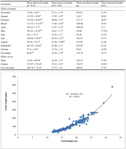
From table 1 and 2, it is appeared that, the total number of fish samples investigated were 290, from which 179 were males, 41 females and 70 fishes immature. The sex ratio male to female were 4.3:1. The mean observed length of male was 18.29 cm at mean observed weight 114.8 g, and mean observed length of female was 19.15 cm at, mean observed weight 133.97 g. The correlation coefficient “r”, which measured the association between Length-weight regression parameters was estimated for all months, males, females and the whole sample are presented in Table 1 and Figures 2, 3 and 4, r seems to be high correlation in all categories r 0.5. The length-weight
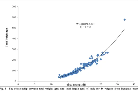
relationships were found significant (P < 0.001) in the all groups. The slope “b” in all categories range between 2.295 in September to 3.208 in August. In January, August and Females the slope “b” close to equal 3, were the categories exhibited isometric relationship, in September, October and Novemberwere slope “b” not equal 3, which the categories exhibited negative allometric relationship and for the other months, males, and both sex showed positive allometric relationship were seen. However, allometry. was very small with coefficients close to 3 and there were no statistically significant differences in slopes or intercepts between males and females. The analysis of variance (Table 2) indicated a high significant effects of months on both total length and total weight, while the sex had no significant effects on the bellow mentioned traits. The general equation for the weight-length relationship for both sexes was: W = 0.03835L2.77
For male was: W = 0.036 L2.74 and For female: W = 0.016 L3.02.
Within columns, means had different superscripts differed significantly (P < 0.05).
Table 2 Mean observed weight and length and calculated weight and length for D. vulgaris from Benghazi coast 2014-2015.
Categories Mean observed weight (g+-S.D.) Mean observed length (cm+-S.D) Mean calculated weight (g) Mean calculated length (cm)
Effect of month
December 71.89 ± 24.9a 15.71 ± 1.8a 78.917 15.19
January 115.55 ± 58.8bc 17.97 ± 2.9b 114.5 18.03
February 155.45 ± 45.05de 20.89 ± 2.3d 173.77 20.07
March 111.55 ± 115.8bcd 17.86 ± 4.8bc 109.46 18.03
April 103.23 ± 7.7bc 17.67 ± 3.3b 109.29 17.3
May 101.81 ± 61.8bcd 16.67 ± 3.7b 93.00 17.223
June 50.1 ± 12.7a 13.63 ± 1.1a 53.24 13.33
July 148.46 ± 54.8cde 20.38 ± 2.5cd 162.27 19.73
August 192.6 ± 53.5ef 22.56 ± 2.08de 215.03 21.68
September 207.25 ± 42.02f 23.90 ± 2.1e 252.30 22.26
October 77.4 ± 18.5a 15.76 ± 1.6a 79.61 14.94
November 94.62ab 18.26 ± 1.9bc 119.70 16.77
Effect of sex
Male 114.8 ± 66.96a 18.29 ± 3.4a 120.25 17.94
Female 133.97 ± 78.10a 19.15 ± 3.8a 136.57 19.017
Over all mean 106.78 ± 73.24 17.53 ± 3.8 106.91 17.52
Fig. 2 The relationship between total weight (gm) and total length (cm) for both sexes for D. vulgaris from Benghazi coast 2014-2015.
W = 0.038L2.722 R² = 0.952
0 100 200 300 400 500 600 700
0 5 10 15 20 25 30 35
Total weight
(g
m)
ر
Fig. 3 The relationship between total weight (gm) and total length (cm) of male for D. vulgaris from Benghazi coast 2014-2015.
Fig. 4 Weight-length relationship for female for D. vulgaris from Benghazi coast 2014-2015.
W = 0.036L2.741 R² = 0.958
0 100 200 300 400 500 600 700
0 5 10 15 20 25 30 35
Total Weight
(gm)
Total length (cm)
W= 0.016L3.016 R² = 0.973
0 50 100 150 200 250 300 350 400 450 500
0 5 10 15 20 25 30 35
Total Weight (g
m)
ر
5. Discussions
The percentage of sex ratio male to female in this a study was 4.3:1, with favor of male. Our results on this study compare with the results of Taieb, et al. 2013, from Tunisia sea, he, recognized that the sex ratio for the species D. vulgaris was 1:1.66, and with Dulcic, et al. 2011, from the Eastern Adriatic Sea, they mentioned 1.22:1, with favor to male, these variation in results me be due to different in locations or types of gears used in captures of this species in its areas ranges. Sadovy and Shapiro, they mentioned that the percentage of males to females varied with size of fish and also by season and months [11].
The length-weight relationships a practical index of the condition of fish. In fisheries studies; the condition factor is an essential biological parameter needed to understand the suitability of the environment for good living of fish [12]. In the present study the Length-weight regression parameters estimated for all months, male, female and both sex were showing different result in slope “b” and showed high correlation coefficient “r” between total weight and total length of species D. vulgaris, presented in table1 and Figs 2, 3 and 4. The length-weight relationships were found significant (P < 0.001) in the all groups. In January, August and Females, were exhibited isometric relationship, in September, October and November were exhibited negative allometric relationship while for the other months, males, and both sex showed positive allometric relationship. However, allometry was very small with coefficients close to 3 and there were no statistically significant differences in slopes or intercepts between males and females. This finding recognized by many authors [4] were suggested that the pattern of weight relative growth may fluctuate over the year according to factors such as food availability, feeding rate, gonad development or spawning period.
In the present study, the value of the exponent “b” for both sex for species D. vulgaris was found to be
(2.8), male (2.7) and female (3.0) which indicated slight positive allometry with both sex and male, while for female which indicate isometric growth. This value was lower for values of (both sex and male) and similar with some values than the values of “b” of D. vulgaris which is estimated by Mahmoud [13] in Abu Qir Bay Egypt, (2.9), in Gulf of Tunis (3.05 both sex, 3.058 for male and 3.078 for female) [14], in the Gulfof Lion (3.123) [15] and in the Egyptian Mediterranean water (3.003) [16]. The differences in b value observed for the species across areas may be attributed to the different atrophic conditions [17]. In fact, the Mediterranean Sea, and the Eastern Basin in particular, is considered as one of the most oligotrophic regions in the world in terms of both primary productivity and chlorophyll a concentrations [18].
References
[1] Richer, W. E. 1975. Interpretation of Biological Statistics of Fish Populations, Department of the Environment Fisheries and Marine Service Pacific Biological Station, Nanaimo, B. C. V 9R5 K6, pp. 266.
[2] Gulland, J. A. 1985. Fish Stock Assessment. A Manual of Basic Methods. Marine Resources Service. Rome, Italy, p. 293.
[3] Ahemed, A. H. 1987. Fish Biology, University of El Basra: pp. 279.
[4] Bagenal, T. B., and Tesch, F. W. 1978. Age and Growth. In: Methods for Assessment of Fish Production in Fresh Waters, third edit. (Bagenal, T. ed.), pp. 101-36. IBP Handbook No. 3. Oxford: Blackwell Scientific Publications.
[5] Ibrahim, S. M. 2013. Study, characterization and biolical study on some species of family Sparidae in Ain El-Ghazala Gulf of eastern Libya. M.Sc. thesis.
[6] Bauchot, M. L., and Hureau, J. C. 1986. Sparidae. In: Whitehead, P. J. P., Bauchot, M. L., Hureau, J. C., Nielsen, J., and Tortonese, E. (Editors). Fishes of the North-eastern Atlantic and the Mediterranean. UNESCO, Paris, 2: 883-907.
[7] Monteiro, P. 1989. La fauneichthyologique de la laguneRia Formosa (Sud Portugal). Repartitionetorganizationspatio-temporelle des communautés: application à l’aménagement des resources.
[8] Santos, M. N. 1997. Icthyofauna of the artificial reefs of the Algarve coast. Exploitation strategies and management of local fisheries. Ph.D Thesis. Universidade do Algarve, UCTRA, Faro, 223 p.
[9] Shakman, E., and Kinzelbach, R. 2007. “Commercial Fishery and Fish Species Composition in Coastal Waters of Libya.” Rostocker Meeresbiologische Beiträge 18: 63-78.
[10] Al-hassan, L. A., and El-silini, O. A. 1999. “Check-list of Bony Fishes Collected from the Mediterranean Coast of Benghazi, Libya.” Revista de Biologia Marina y Oceanografia 34: 291-301.
[11] Sadovy, Y., and Shapiro, D. Y. 1987. “Criteria for the Diagnosis of Hermaphroditism in Fishes.” Copeia 1987: 136-56.
[12] Le Cren, E. D. 1951. “The Length Weight Relationship and Seasonal Cycle in gonad weight and Condition in the Perch (Perca fluviaittlis).” J. Anim. Ecol. 20: 201-19. [13] Mahmoud, H. H., Osman, A. M., Ezzat, A. A., and Salah,
A. M. 2010. “Biological Status and Management of
Diplodus vulgaris (Geoffroy Saint-Hilaire, 1817) in Abu Qir Bay, Egypt.” Egyptian, Jou. of Aquatic Res. 36 (1): 115-22.
[14] Mouine, N., Mohamed, H., and Nadia, M. C. 2010. “Age
and Growth of Diplodus vulgaris (Sparidae) in the Gulf of Tunis.” Cybium 34 (1): 37-45.
[15] Man Wai, R., and Quignard, J. P. 1982. “The Seabream
Diplodus sargus (Linne 1758) in Gulf of Lion: Growth of the Seabream and Characteristics of Landings from the Commercial Fishing Grounds of Sete and Grau-du-Roi.Rev.”
Trav. Inst. Peches Marit. Nates 46 (3): 173-19.
[16] El-Maghraby, A. M., and Botros, G. A. 1981. “Maturation, Spawning and Fecundity of Two Sparid Fish, D. sargus, D. vulgaris and Geoffer Bull.” Nat. Inst. of Oceanography and Fisheries, ARE 8 (2): 51-67. [17] Chilari, A., Petrakis, G., and Evaggelos, T. 2006.
“Aspects of the Biology of Blackspot Seabream (Pagellus bogaraveo) in the Ionian Sea, Greece.” Fish. Res. 77: 84-91.
[18] Azovy, Y. 1991. “Eastern Mediterranean: a Marine Desert?” Mar. Pollut. Bull. 23: 225-32.
[19] Dulčić, J., Pallaoro, A., Matić-Skoko, S., Dragičević, B., Tutman, P., Grgičević, R., Stagličić, N., Bukvić, V., Pavličević, J., Glamuzina, B., and Kraljević, M. 2011. “Age, Growth and Mortality of Common Two-banded Seabream, Diplodus vulgaris (Geoffroy Saint-Hilaire, 1817), in the Eastern Adriatic Sea (Croatian coast).”
Journal of Life Sciences 10 (2016) 66-76 doi: 10.17265/1934-7391/2016.02.002
Genotoxic Effects in Mice Exposed to Radon Emissions
in Indoor Conditions. Comparison between
in utero
and
Neonatal Exposures
Cristiano Foschi1, Manuel Luís Orta2, Licia Radicchi3, Germana Szpunar1 and Mauro Cristaldi1
1. Department of Biology and Biotechnology Charles Darwin, Faculty of Mathematical, Physical and Natural Sciences, University of Rome, Rome 00161, Italy
2. Department of Cell Biology, Faculty of Biology, University of Seville, Seville 41012, Spain 3. Civic Museum of Zoology, via U. Aldrovandi 18, Rome 00197, Italy
Abstract: The purpose of this study was to develop a biological model to evaluate the genotoxic effects of natural emissions of Radon-222 and its decay products. To this aim, mice of the Swiss CD1 strain were exposed to Radon for different periods (adult life, early postnatal and in utero exposure) and two simple but accurate mutagenicity tests (Micronucleus test and the Comet assay) were applied to the peripheral blood of mice. The study was carried out in two small towns in Latium region—Italy, where radon pollution is notoriously present due to the volcanic soils. One experiment was carried out in the cellar of a house in Ciampino (Rome) and two experiments were performed in an old cellar in Vetralla (Viterbo). The results showed that in all mice groups exposed to natural emissions of radon and its decay products, the micronucleated erythrocytes frequency (ME) was significantly higher than that observed in the mice control. The single cell gel electrophoresis (Comet assay) was performed in lymphocytes of adult mice in the last experiment. The results for this test also show that DNA damage was higher than in the cells of the mice control and the cells of mice exposed for a shorter period of time. To confirm these findings, the single cell gel electrophoresis (Comet assay) was performed in lymphocytes of adult mice in the last experiment. Similarly, this result could be linked to a greater sensitivity of neonatal mice to radon emissions compared with intrauterine mice. Further investigations on the effects of radon and its decay products during the intrauterine life and the first neonatal period should be performed to better clarify its genotoxic activity.
Key words: Radon, genotoxicity, DNA damage, micronucleus test, comet assay.
1. Introduction
Radon is a radioactive noble gas, chemically inert, decay product of Uranium-238. It is classified by WHO/IARC as group 1 carcinogen. Home (indoor) exposure to short lived radioactive disintegration products of Radon-222 is responsible for about half of all non-medical exposure to ionizing radiation [1]. Uranium-238 is present throughout the earth’s crust, but environmental exposure to Radon-222, and its decay products, is especially stronger in dwellings located in areas where the subsoil is rich in Uranium
Corresponding author: Cristiano Foschi, Ph..D., research fields: radon, genotoxicity, natural radioactivity, DNA damage and mutagenicity testing.
or Thorium. Radon rises up from the soil surface (some building materials emit large quantities) and tends to accumulate in confined spaces. In addition it can enter buildings through the called “chimney effect” due to pressure imbalance that is created for the highest temperature of the air in confined spaces. This problem affects mainly basements and floor plans, and therefore people who work in tunnels, underpasses and caves (catacombs guides, bank employees, etc.) are continuously exposed to these radioactive isotopes.
Radon has a half life of 3.8 days, allowing it to diffuse from the soil into the air before decaying by emission of α particle into a series of its short lived radioactive progeny. Two of these, Po-218 and Po-214, also decay by emitting α particles.
D
Most of the inhaled Radon is immediately exhaled, however it tends to be deposited on the bronchial epithelium, thus exposing cells to irradiation [2]. Since the beginning of the last century a relation between exposure to high radon concentration and lung cancer was observed [3, 4]. Studies of exposed miners have consistently confirmed associations between radon and lung cancer [5, 6]. However, results obtained on the biological effects are hard to explain, because of the differences in several parameters, such as duration and periodicity of exposures, concentration values of radon and products decay, synergic effects of tobacco smoke, etc. Genotoxic properties of Radon have been investigated because they are important in order to understand the events that may involve radon to the onset of neoplasia in cytogenetic studies [7-11].
In this study we present data that demonstrate that Radon exposures in two Italian areas cause genotoxicity in vivo as measured with two standard techniques. Furthermore, our data also suggest that animals in the neonatal period are more sensitive to Radon as compared to fetuses [12, 13].
2. Materials and Methods
2.1 Study Sites: Experiments were Carried out in Ciampino (Rome) and Vetralla (Viterbo) (Fig. 1)
2.1.1 Ciampino Experimental Design (13-09-2007/05-10-2007)
Two females CD-1 Swiss in advanced pregnancy (around the 15th gestation day), caged with water and food ad libitum were placed in the cellar of a building. Within three days of the start of the experiment, both females gave birth to 13 newborns. In total 26 newborn mice were exposed to radon gas for 21 days (three days of intrauterine exposure and 18 days of exposure after birth).
2.1.2 Vetralla Experimental design 1st experiment (25-12-2007/29-01-2008):
Three pairs of adult CD-1 Swiss, were placed in three cages. A fourth cage contained the four adult males.
All cages contained water and food ad libitum. The cages were placed in a cellar, six meters below road level. The three pairs gave birth to two, 15 and 11 mice, respectively. In total 28 newborn mice were exposed to radon for 23 days (18 to 19 days of intrauterine exposure and four to five days of exposure after birth).
2nd experiment (18-12-2009/20-01-2010):
Eight adult females CD-1 Swiss, were placed in two cages (four mice per cage), with water and food ad libitum. The cages were placed in a cellar, six meters below the road level, and exposed to radon for about 33 days. The experiments were performed six meters below ground level in Vetralla, and about two meters below ground level in Ciampino.
2.2 Determination of Radon-222 Activity
Ciampino cellar: Radon-222 activity measurements were carried out for over 22 days in the proximity of the cages, by an active detector (Radon Scout made by SARAD GmbH, Dresden, Germany).
Vetralla cellar: Radon-222 activity was measured for by an active detector (AWARE Corporation RADIM 5 made by Plch Smm, Czech Republic) and CR 39 passive detectors provided and analyzed by U-Series, Bologna, Italy.
In both instruments (active detectors) the concentration of radon is determined by measuring the
α-activity of the decay products of the conversion of radon, Polonium-218 and Polonium-214, collected from the detection chamber on the surface of a semiconductor detector by an electric field. The only difference in these two detectors is the time interval used between measurements.
Radon concentrations were calculated by the laboratory “U-Series” (Bologna, Italy).
2.3 Genotoxicity Testing
between in utero and Neonatal Exposures
Fig. 1 Map of Latium region; Ciampino is indicated by outlined arrow, Vetralla by solid arrow (source: www.tuttocitta.it).
damage prior to exposure. These mice were immediately tested again after the exposure period. Control mice (newborns and foetuses) of the same strain and age were held in stabulary and tested in the same manner at the end of the exposure time only.
Micronucleus test: smears were prepared by blood samples collected by caudal vein puncture of each animal, avoiding any useless suffering and pain. Slides were coded, fixed in absolute methanol and stained with the May-Grunwald-Giemsa stain. Micronuclei (MN) were scored blindly by the same
analyst at 1,000x magnification and micronuclei frequencies were determined counting 2,000 erythrocytes per animal.
Comet assay: blood samples were collected by caudal vein puncture, as before described, and placed in Eppendorf tubes (1 mL). Heparin was used as an anticoagulant and DMSO (10%) was added before freezing.
Slide preparation: regular slides were coated with a 1% solution of standard agarose in distilled water, by immersing vertically for 2 s and air-drying to solidify the agarose. Once the slides were dry and totally transparent, they were kept at 4 °C and used up to 1 month after preparation. We employed a modification [14] of the protocols described by Singh et al. [15] and Fairbairn et al. [16]. Only 40-100 μL of cell solution was embedded in a 0.7% low melting agarose solution in PBS and immediately pipetted onto the coated slides and then a coverslip was placed on. The slides were incubated at 4 °C for 10 min. Coverslips were removed and a third (low melting) agarose layer was added, together with new coverslips. Slides were again incubated at 4 °C for 10 min. Coverslips were finally removed and cells were immersed in lysis solution (10 mM Tris-HCl, 2.5 M NaCl, 100 mM Na2-EDTA, 0.25 M NaOH, 1% (v/v) Triton X-100
and 10% (v/v) DMSO, pH 12.0) for 1 h at 4 °C in the dark.
Electrophoresis: in order to unwind the DNA, the slides were incubated for 20 min in electrophoretic buffer containing 1 mM Na2-EDTA and 300 mM
NaOH, pH 12.8 (Alkaline conditions). Electrophoresis was carried out at 1 V/cm for 20 min. Slides were then neutralized with 3 × 5 min washes of 0.4 M Tris-HCl pH 7.5 to remove alkali and detergent. After that, cells were stained with the fluorochrome 4' 6-diamidino-2-phenylindole (DAPI) in Vectashield (mounting medium for fluorescence H-1000, Vector Laboratories). Slide scoring: DNA damage was analysed using the Comet Score program (an online free Comet scoring software web). Two parameters were estimated for each Comet: (1) DNA damage (percentage migrated DNA in the tail), and (2) tail moment (tail length × tail intensity or percent
migrated DNA). Five different classes of DNA damage were established following classification given by Anderson et al. [16]. Class 1 corresponded to cells showing DNA damage between 0 and 5%, class 2 (5-20%); class 3 were cells with DNA damage between (2-40%); class 4 (40-95%); and class 5 (95-100%), which corresponds to cells with the highest damage or totally damaged cells. For each experimental point at least 324 Comets were measured.
2.4 Statistical Analysis
Micronucleus test: since some of the variables were not normally distributed (Lilliefors test, P < 0.05), we used nonparametric tests. Medians were analysed by Mann-Whitney U-test.
Comet assay: Mann-Whitney test and χ2 (chi-square test) have been used for statistical evaluation.
All statistical analyses were carried out using STATISTICA 6.0 package (StatSoft, Tulsa, OK, USA).
3. Results and Discussion
3.1 Exposures
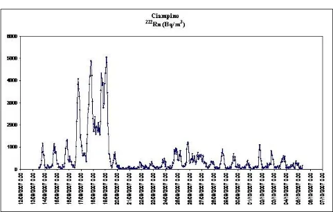
Ciampino site: Figure 2 shows the 222Rn concentrations measured using electronic detector Radon Scout in continuum. The mean concentration of the entire period of the exposition of the newborns was 562 Bq/m3. The graphic shows large yet short variations of radon activity, ranging from the maximum value of 5,054 Bq/m3 and the minimum value (0 Bq/m3). Total exposure at the end of period was 260 kBq h/m3.
between in utero and Neonatal Exposures
Fig. 2 Graph showing the trend of the concentration of 222Rn (Bq/m3) monitored by the active detector Radon Scout in Ciampino from 12/09/2007 to 07/10/2007.
period was 1,090 kBq h/m3. Total exposure for adult mice (entire period of 35 days) was 1,700 kBq h/m3.
2nd experiment: 222Rn concentrations were measured using just passive detectors (CR-39). The exposure was calculated every 10 days (Table 1). The mean concentrations are included between 745 Bq/m3 to 2,100 Bq/m3. Total exposure after the last ten days was 200 kBq h/m3, after twenty days 560 kBq h/m3 and, since the start to the end of the period, was 1,160 kBq h/m3.
With regards to the experiments of newborns and foetuses (Vetralla) the entire exposure period (about 25 days) consisted of about 19 days of intrauterine exposure and five to six days of exposure after birth. These data were compared with those obtained in newborn mice from the cellar in Ciampino exposed to
222Rn for three to four days
in utero and 18 days of postnatal exposure (about 22 days in total). The mice located in the Vetralla cellar were exposed to a 222Rn concentration (1,090 kBq h/m3) almost four times higher compared with the mice exposed in Ciampino’s cellar (260 kBq h/m3).
3.2 Micronucleus Test
Micronucleus test was carried out on newborn mice (N = 26 from Ciampino and N = 28 from Vetralla) and adult mice (N = 18) from two experiments carried out in Vetralla.
Ciampino site: Table 1 shows the results obtained applying peripheral blood micronucleus test in the newborn mice exposed in Ciampino cellar and in the control mice. It was observed that the frequency of micronucleated erythrocytes is significantly higher in
the exposed group compared with the control group (P < 0.0001).
Vetralla site: Table 2 shows the mean frequencies of peripheral blood micronucleus test in all mice offspring born in Vetralla cellar and in the control offspring. It was observed that the frequency of micronucleated erythrocytes is significantly higher in the exposed group compared with the control group (P < 0.05).
Vetralla 1st experiment: Table 3 shows the mean frequencies of peripheral blood micronucleus test before exposure and after 35 days in the Vetralla cellar. It was observed that the frequency of micronucleated erythrocytes is significantly higher in the exposed group compared with the control group (P < 0.05).
Vetralla 2nd experiment: Table 4 shows the mean frequencies of peripheral blood micronucleus test before exposure and after 33 days in the Vetralla cellar. It was observed that the frequency of micronucleated erythrocytes is significantly higher in the exposed group compared with the control group (P < 0.001).
In the experiment carried out in Ciampino, the genotoxic damage observed in newborn mice exposed to a low indoor radon concentration (300 kBq h/m3) may be related to the period in which the animals were exposed. It should be noted that in this case the females were exposed on the 15th the day of pregnancy. Therefore the newborn mice were exposed for fewer days during the intrauterine life (4-5) and for 18 days after birth, compared with the mice in the Vetralla cellar which were exposed for the whole intrauterine phase and only for few days (4-5) after birth.
Table 1 222Rn concentrations measured by passive detectors (CR-39) and relative exposures.
Vetralla 2ndexperiment
Time of exposure Concentrations 222 Rn [Bq/m3]
Exposure
[kBq h/m3] Total exposure [kBq h/m3]
18/12/2008-29/12/2008 745 ± 170 200 ± 40 200 ± 40
29/12/2008-09/01/2009 1,500 ± 350 360 ± 80 560 ± 90
between in utero and Neonatal Exposures
Table 2 Mean frequencies ± SD of micronucleated erythrocytes in newborn mice exposed in Ciampino cellar. N = number of animals; ME = Micronucleated Erythrocytes; E = Erythocytes; Control = mice not exposed (from stabulary at the Sapienza University, Rome); significance respect to control: b = P < 0.01; d = P < 0.0001.
Ciampino
N ME/1,000 E Exposure [kBq h/m3]
Control 9 0.83 ± 0.66 -
Exposed 26 3.65d ± 2.27 260
Vetralla
N ME/1,000 E Exposure [kBq h/m3]
Control 18 1.25 ± 0.7 -
Exposed 28 2.34b
± 1.49 1,090
Table 3 Mean frequencies ± SD of micronucleated erythrocytes in adult mice exposed in Vetralla cellar. N = number of mices; ME = Micronucleated Erythrocytes; E = Erythocytes; Control = blood samples before exposure; significance respect to control: a = P < 0.05.
Vetralla 1st experiment
N Male/female ME/1,000 E Exposure [kBq h/m3]
Control (before exposure) 10 7/3 0.75 ± 0.49 -
Exposed 10 7/3 1.6a ± 0.7 1,700
Table 4 Mean frequencies ± SD of micronucleated erythrocytes in adult mice exposed in Vetralla cellar. N = number of mice (females); ME = Micronucleated Erythrocytes; E = Erythocytes; Control = blood samples before exposure; significance respect to control: c = P < 0.001.
Vetralla 2nd experiment
N ME/1,000 E Exposure [kBq h/m3]
Control (before exposure) 8 0.94 ± 0.56 -
Exposed 8 2.25c ± 0.46 1,160
3.3 Comet Assay
In the present study we have made use of the rapid method applicable to mammalian lymphocytes, which do not need to be isolated with the potentially cytotoxic drug Ficoll, as previously described by Daza et al. [13]. As we can see in Table 5, DNA damage assessed by the Comet assay in mice after final
exposure (1,160 kBq h/m3) was statistically significantly higher (Mann-Whitney test) than that observed in control samples (taken before exposure). Significant statistical differences were observed
considering both the parameters scored (percent of damage DNA in the Comet tail, and tail moment of the Comets).
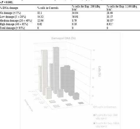
Another statistical analysis (χ2 or chi-square test) has been carried out considering the five classes of DNA damage reported by Anderson et al. [17]. Table 6 and figure 4 show the percentages of cells for both
control mice and exposed mice, belonging to the various classes of damage (absent, low, medium, high and total).
Data obtained from the experiments in both the Ciampino and Vetralla cellars show that perinatal exposure to radon emissions induces a significant increase in micronuclei frequencies (ME/1,000E) both in newborn mice and in mice exposed during intrauterine phase.
Some differences in the two experiments should be noted: in Ciampino, the exposure was almost totally neonatal (from birth until 18 days after) compared with the exposure in Vetralla which was mainly intrauterine (about 19 days).
Table 5 Damage as assessed by the Comet assay. N = number of mice; n.a. = not available; significance respect to control: a = P < 0.05.
N Number of cells DNA damage (%) Tail moment
Control (before exposure) 3 324 9.98 ± 2.82 6.40 ± 3.24
Exposure 200 [kBq h/m3] 5 523 9.36 ± 3.32 8.98 ± 4.99
Exposure 1,160 [kBq h/m3]
8 852 16.29 ± 4.89a 21 ± 13.86a
Table 6 Percentages of cells with DNA damage absent, low, medium, high, and total; significance respect to control: c = P < 0.001.
% DNA damage % cells in Controls % cells for Exp. 200 kBq h/m3
% cells for Exp. 1,160 kBq h/m3
No damage (< 5%) 32.1 34.04 28.64
Low damage (5 ÷ 20%) 54.32 56.98 33.57
Medium damage (20 ÷ 40%) 12.96 8.79 30.87c
High damage (40 ÷ 95%) 0.62 0.19 6.92 c
Total damage (> 95%) 0 0 0
Fig. 4 Histogram of percentages of cells with DNA damage absent, low, medium, high, and total.
The difference observed between the two groups in the tests could be due to the differing period of exposure to radon and its decay products, indicating a higher degree of susceptibility during the postnatal period.
between in utero and Neonatal Exposures
concentrations of radionuclides in embryonic tissues are almost systematically lower than the concentrations found in the tissues of the mother, and that the first part of a newborn’s life (breastfeeding) is a period in which the absorbed dose is higher.
The same results were observed in the experiments performed with adult mice in the Vetralla cellar. Exposure to radon emissions induces a significant increase in micronuclei frequencies in peripheral blood erythrocytes (ME/1,000E). Final exposure, after more than thirty days (1stexperiment: 1,700 kBq h/m3; 2nd experiment: 1,160 kBq h/m3) caused a statistically significantly higher frequency of ME than that observed in the control samples (taken before exposure).
The results highlighted by the Micronucleus test were confirmed in the second experiment carried out on adults, through the application of the Comet assay. This test, has, in fact underlined a statistically significant increase in DNA damage after exposure to radon than the damage detected in the control samples (taken before the exposure).
4. Conclusions
In conclusion, the work presented here confirms, on the basis of experimental evidence conducted on mice whose the biological model is perfectly comparable to the human species as already observed in previous studies [21-25], the effects caused by prolonged exposure to radon gas emissions.
In particular, the present study aims to highlight that workers in certain subterranean environments (bank vaults, catacombs, etc.), individuals living in homes constructed of tufaceous material and those who have settled in volcanic areas are all subject to potential genetic risks.
This study has shown a particular sensitiveness to radon and its decay products that is not as strong in murine embryos, protected by the placental tissues but appears in newborn mice, which already display genetic damage from exposure levels (260 kbq/m3)
lower than those that cause genetic damage in adults and embryos (about 1,000 kbq/m3). It would therefore be appropriate to carry out further studies on this issue, in order to propose the most suitable prevention strategies in terms of social-health.
Indoor radon levels are affected by the soil composition under and around the buildings, and by the easiness with which radon enters the houses. Homes that are very close to each other can have different indoor radon levels. In addition, precipitation, barometric pressure, climate change parameters, hydrogeological phenomena and other factors can cause radon levels to vary from month to month or day to day, which is why both short- and long- term tests are available. The graphics showing the measurements of radon concentration registered in the cellars can be a good illustration of the varying of the radon levels in a confined environment. However, exposure obtained in the two experiments, can be used to say that the area of Vetralla could due to higher concentrations. Of course it depends by the soil composition of the area.
5. Conflict of Interests
The authors declare no conflict of interests regarding the publication of this paper.
Acknowledgments
Luisa Anna Ieradi for kind suggestions and helpful instruction; Doctorate School of Industrial and Environmental Hygiene directed by Prof. I. Figà-Talamanca; PRIN 2012 project “Effetti dei cambiamenti climatici sulle microteriocenosi terrestri” (Effects of climate change on terrestrial microtheriocoenoses); Prof. P. Brandmayr. Thanks to Zach Butcher for the careful proof reading.
References
[1] UNSCEAR (United Nations Scientific Committee on the Effects of the Atomic Radiation), “Sources and Effects of Ionizing Radiation,” United Nations, New York, 2000.
[2] Ruano-Ravina, A., Ruosteenoja, E., Schaffrath, R. A., Tirmarche, M., Tomáek, L., Whitley, E., Wichmann, H. E., and Doll, R. 2005. “Radon in Homes and Risk of Lung Cancer: Collaborative Analysis of Individual Data from 13 European Case-control Studies.” British Medical Journal 330 (7485): 223.
[3] Schuttmann, W. 1993. “Schneeberg Lung Disease and Uranium Mining in the Saxon Ore Mountains (Erzg ebirge).” American Journal of Industrial Medicine 23 (2): 355-68.
[4] Greenberg, M., and Selikoff, I. J. 1993. “Lung Cancer in the Schneeberg Mines: a Reappraisal of the Data Report.” The Annals of Occupational Hygiene 37 (1): 5-14.
[5] IARC—International Agency for Research on Cancer, “Man-made Mineral Fibres and Radon. IARC Monographs on the Evaluation of Carcinogenic Risks to Humans 43.” IARC, Lyon, 1998.
[6] Darby, S. C., Whitely, E., Howe, G. R., Hutchings, S. J., Kusiak, R. A., Lubin, J. H., Morrison, H. I., Tirmarche, M., Tomásek, L., Radford, E. P., Roscoe, R. J., Samet, M. J., and Yao, S. X. 1995. “Radon and Cancers Other Than Lung Cancer in Underground Miners: a Collaborative Analysis of 11 Studies.”
Journal of the National Cancer Institute 87 (5): 378-84.
[7] Nelson, S. L., and Grosovsky, A. J. 1995. “Evidence for a Gene Distal to HPRT which Restricts the Recovery of Large Deletions.” Environmental Molecular Mutagenesis 25: 39-43.
[8] Schlegel, R., and Mac Gregor, J. T. 1982. “The Persistence of Micronuclei in Peripheral Blood Erythrocytes: Detection of Chronic Chromosome Breakage in Mice.” Mutation Research 104: 367-9. [9] Rommens, C. C., Ringeard, C., and Hubert, P. 2001.
“Exposure of Red Bone Marrow to Ionising Radiation from Natural and Medical Sources in France.” Journal Radiological Protection 21: 209-19.
[10] Hellmann, B., Friis, L., Vaghef, H., and Edling, C. 1999. “Alkaline Single Cell Gel Electrophoresis and Human Biomonitoring for Genotoxicity: a Study on Subjects with Residential Exposure to Radon.”
Mutation Research 442: 121-32.
[11] Fukutsu, K., Ya mada, Y., Zhuo, W., and Koizumi, A. 2005. “Induction of Micronuclei in Rat Tracheal Epithelial Cells Following Radon Exposure at Air-liquid Interface Culture.” International Congress Series 1276: 251-3.
[12] Udroiu, I., Cristaldi, M., Ieradi, L. A., Bedini, A., Giuliani, L., and Tanzarella, C. 2006. “Clastogenicity and Aneuploidy in Newborn and Adult Mice Exposed to 50 Hz Magnetic Fields.” International Journal of Radiation Biology 82 (8): 561-7.
[13] Ieradi, L. A., Cristaldi, M., Ermenegildi, A., La Barbera, L., Radicchi, L., Renzopaoli, F., Esposito, M., and Lombardi, S. 2008. “Mutagenic Effects in Mice Exposed to Radon-222 Emissions in Latium Region (Italy).” Fresenius Environmental Bulletin 17 (9b): 1420-5.
[14] Daza, P., Torreblanca, J., and Moreno, F. J. 2004. “The Comet Assay Differentiates Efficiently and Rapidly between Genotoxins and Cytotoxins in Quiescent Cells.” Cell Biology International 28: 497-502.
[15] Singh, N. P., Mc Coy, M. T., Tice, R, R., and Schneider, E. L. 1988. “A Simple Technique for Quantitation of Low Levels of DNA Damage in Individual Cells.” Experimental Cell Research 175: 184-91.
[16] Fairbairn, D. W., Olive, P. L., and O'Neill, K. L. 1995. “The Comet Assay: a Comprehensive Review.”
Mutation Research 339: 37-59.
[17] Anderson, D., Yu, T. W., Phillips, B. J., and Schmezer, P. 1994. “The Effect of Various Antioxidants and Other Modifying Agents on Oxygen-radical-generated DNA Damage in Human Lymphocytes in the COMET Assay.” Mutation Research 307: 261-71.
[18] ICRP, “Doses to the Embryos and Fetus from Intakes of Radionuclides by the Mother. ICRP Publicationn 88.” Annals of the ICRP 31 (1-3) (Oxford Elsevier Science), 2001.
[19] Stather, J. W. 2003. “Dose Coefficients for the Embryo and Foetus following Intakes of Radionuclides by the Mother.” Journal of Radiological Protection 22: 7-24. [20] Kendall, G. M., Fell, T. P., and Harrison, J. D. 2009.
between in utero and Neonatal Exposures
[21] Little, C. C. 1937. “US Science Wars against an Unknown Enemy: Cancer.” Life 2: 11-7.
[22] MacKey, B. E., and Mac Gregor, J. T. 1979. “The Micronucleus Test: Statistical Design and Analysis.”
Mutation Research 64 (3): 195-204.
[23] Waterston, R. H., et al. 2002. “Initial Sequencing and Comparative Analysis of the Mouse Genome.” Nature
420: 520-62.
[24] Paigen, K. 2003. “One Hundred Years of Mouse Genetics: an Intellectual History. I. The Classical Period (1902-1980).” Genetics 163: 1-7.
doi: 10.17265/1934-7391/2016.02.003
Stochastic Lattice gas Cellular Automata Model for
Epidemics
Ariel Félix Gualtieri and Juan Pedro Hecht
Department of Biophysics, Faculty of Dentistry, University of Buenos Aires, Buenos Aires C1122AAH, Argentina
Abstract: The aim of this study was to develop and explore a stochastic lattice gas cellular automata (LGCA) model for epidemics. A computer program was development in order to implement the model. An irregular grid of cells was used. A susceptible-infected-recovered (SIR) scheme was represented. Stochasticity was generated by Monte Carlo method. Dynamics of model was explored by numerical simulations. Model achieves to represent the typical SIR prevalence curve. Performed simulations also show how infection, mobility and distribution of infected individuals may influence the dynamics of propagation. This simple theoretical model might be a basis for developing more realistic designs.
Key words: Disease spread, people movement, epidemic model, stochastic lattice gas cellular automata.
1. Introduction
In the large majority of studies involving population dynamics, such as the spread of epidemics, direct experimentation is often not feasible. That is why formal models can offer a great help, providing a framework for exploring these scenarios. Mathematical models of epidemics are formal designs that capture the dynamic behaviour of spread of infectious diseases [1, 2].
The first step to define an epidemic model is to classify individuals of the population into different categories corresponding to possible states for the disease under study. According to this grouping, parameters are defined to represent the transition of individuals between these categories over a period of time. The aim then is to study the evolution of the system over time [3]. The choice of which states to include in a model depends on the characteristics of the particular disease being investigated and the purpose of the model. Acronyms for epidemic models are often based on the flow patterns between the different states considered [4]. For example, in a
Corresponding author: Ariel Félix Gualtieri, Ph.D., research fields: applied mathematics, epidemiology and biostatistics.
susceptible-infected-recovered (SIR) type model, individuals can be in one of three states; they are susceptible (S) and can catch the disease, infected (I) and can spread the disease, or recovered and immune (R). The SIR scheme is representative of diseases in which individuals develop immunity, such as influenza [5-7].
The dynamics of current models of epidemics rarely lead to analytical solutions. To achieve this, it would be necessary simplifications to reduce the formal complexity of the models, which would reduce their representativity [8]. Thus, despite its formal nature, the results provided by current epidemiological mathematical models are often analyzed in a qualitative way from numerical computer simulations. The difficulty of including all relevant factors, the imprecise measurement of biological and behavioural variables, and the extreme sensitivity of many non-linear systems to small changes in parameter values are frequently insurmountable obstacles to accurate quantitative prediction [9]. Thus, qualitative results can provide a coherent framework of analysis that is more efficient than simple intuition, helping in the planning of health policies.
Both deterministic and stochastic models are used
D
to describe the transmission dynamics of epidemics. The deterministic models based in systems of equations, often lead to powerful qualitative results with important threshold behaviour. They also lead to simpler mathematical problems than the stochastic ones. Work on deterministic models has therefore dominated strongly over work on stochastic models [10]. However, deterministic models are not appropriate when population size is small and stochastic factors play a major role [9]. There are a number of ways to allow the events in a model to be influenced by chance, but the most common and rigorous method is Monte Carlo simulation, where a set of possible events is defined with a probability attached to each of them. A random number generator is then used to calculate which of the range of possible events it will be [9].
Classical epidemic models have tended to minimize geographic heterogeneity and related spatial aspects of spread of infectious diseases. However, spatial epidemic models have become more important in recent years [11-13]. Spatial models of infectious disease transmission provide the only framework in which knowledge of the location of hosts and their movement patterns can be combined with a description of the infection process and the disease natural history to investigate observed patterns and to evaluate alternative intervention options [14].
The significant development of computer technology during the last decades has allowed the design of mathematical computer models that supply explicit spatial representations of complex systems. One example is the cellular automata (CA) models. They are dynamic simulation models defined by spatially arranged mathematical cells, which are updated in discrete steps according to a set of rules. The nature of these update rules determines whether the model will have a deterministic or a stochastic behaviour [15]. In recent years the development of CA models for the spread of infectious diseases has
increased. Both deterministic [16-18] and stochastic [19-21] designs have been developed.
In CA models for epidemics, each cell can be considered as an individual or a small subpopulation [22-24]. Alternatively, each cell may represent an area (patch) occupied by a certain number of individuals who can interact within the cell and move to other cells [17, 19, 25]. This will be the case in the model presented in this work. A CA whose cells contain particles that interact within the cells is called lattice gas cellular automata (LGCA) [19]. As computer technology continues to improve, the development of epidemiological models of CA also increases. Although these models do not provide analytical solutions, they help to understand the spatial dynamics and to identify what factors might be relevant to the spread of epidemics in spatially structured populations [26].
The aim of the present work is to develop and explore a stochastic LGCA model that can be a basis for studying the spread and control of epidemics and their relation to the spatial distribution and mobility of the population.
2. Materials and Methods
The model was implemented in an original computer program developed by the authors of the present work in Delphi® platform. The software includes the Delphi-Component Tmesh for representing irregular grids in cellular automata simulations [27]. The model presents a two-dimensional grid of 900 cells with different shapes incorporated in this component (Fig. 1). If two cells are adjacent, they are considered neighbours. Thus, each cell can be surrounded by a different number of neighbours. In each cell there is a given number of individuals who can move between neighbouring cells.
Fig. 1 Two-dimensional grid of 900 cells included in the Delphi-Component Tmesh [27] and used in the model of the present work.
or recovered (R). For each cell i, the model includes the following events influenced by chance: infection, recovery and displacement to a neighbouring cell selected at random. A state transition parameter is assigned to each of these events. The authors named β, γ and δ to parameters for infection, recovery and displacement, respectively. These parameters have the same value in all cells. The value of each parameter is proportional to the probability of occurrence of the corresponding process. In addition, it is considered that the net rate at which infection is acquired in each cell i also depends on the number of encounters between susceptible and infected in that cell. Thus, for each cell i the net rate of infection is proportional to βSiIi, where Si and Ii are the number of susceptible and
infected individuals placed in the cell i, respectively. The system is updated at discrete intervals of time (epochs), incorporating random effects by using Monte Carlo method according to the manner described below. The parameters that affect individuals of each state define a range proportional to its magnitude in the interval (0, 1). For each epoch a random number generator built into the program produces values within this range, which allows
selecting the event that individuals of each state will experience. Thus, for each epoch, individuals can experience one of the following events: change of state, displacement to a neighbouring cell selected at random or remain unchanged. Finally, the number of individuals in each state per cell is updated and the simulation time is incremented by one epoch. The program allows to set the initial number of individuals in different states by cell. When a simulation is completed, the program generates an analytical record of the number of individuals in the states S, I and R for each cell and for the entire system as a function of simulation time in epochs. The application also provides visual representations of the spread of the outbreak on the lattice of cells through bitmaps.
The dynamics of the model was explored by computer numerical simulations. Arbitrary values were assigned to initial conditions and to state transition parameters.
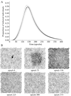
3. Results
Fig. 2 Evolution of the epidemic in the benchmark case. (A) Proportion of infected individuals as a function of time. Mean (black markers) and mean + standard deviation (gray markers) of 10 repeat simulations are displayed. (B) Spatial pattern of the infected individuals for different times in a typical simulation. The colour of each cell is related to the number of infected individuals placed there: white correspond to zero infected individuals and a darker shade of gray indicates a larger number of them. The arrow indicates the cell in which infected individuals are placed at epoch 0.
the figure legend. It can be seen how the evolution of epidemics on the lattice is in agreement with the obtained prevalence curve.
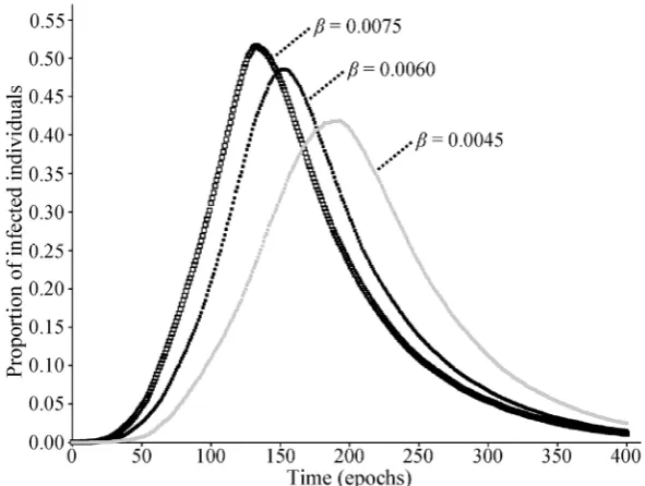
The authors explored the sensitivity of the system to parameters β and δ by varying them one by one, and keeping other conditions as in the benchmark case. These parameters might be affected by health control strategies. For example, some measures implemented during an influenza epidemic can cause a direct reduction in the rate of infection of
Fig. 3 Influence of β on the evolution of prevalence. Three values were tested: β = 0.0075 (open black markers); β = 0.0060 (solid black markers); β = 0.0045 (solid gray markers). Other conditions remain the same as the benchmark case. A typical simulation is shown for each value.
Fig. 4 Influence of δ on the evolution of prevalence. Three values were tested: δ = 0.1500 (open black markers); δ = 0.0750 (solid black markers); δ = 0.0375 (solid gray markers). Other conditions remain the same as the benchmark case. A typical simulation is shown for each value.
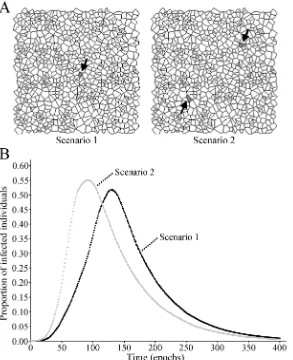
Finally, the authors show that the initial distribution of infected individuals can influence the behaviour of the system. Two initial scenarios were compared: a central cell occupied by six infected individuals and two cells with three infected individuals in each one (Fig. 5a); all other conditions remained as in the benchmark case. The prevalence curve is more steep
during the ascending phase and a higher peak prevalence is reached when infected individuals are distributed in two cells than when they are located in one cell at the beginning of the simulation (Fig. 5b).
4. Discussion
Fig. 5 Influence of the initial distribution of infected individuals on the evolution of prevalence. Two initial scenarios were compared. Scenario 1: a central cell occupied by six infected individuals. Scenario 2: two cells with three infected individuals in each one. (A) Visual representation of each scenario at epoch 0. The arrows indicate the cells in which infected individuals are placed at epoch 0. (B) Typical prevalence curves obtained to scenario 1 (black markers) and scenario 2 (gray markers).
theoretical basis for the study of different scenarios where it is important to assess the mobility and distribution of individuals among several areas. For example, it could be an initial design for the investigation of the spread of outbreaks of some diseases (e.g., influenza) in megacities, where the restriction on population mobility could be a public health measure implemented by governments [30]. Each cell in the system (patch) could represent a given area of the city. On the other hand, the model allows to set the initial distribution of infected individuals, which could be a point of interest for governments in order to evaluate the impact of bioterrorist attacks in megacities. In recent years, bioterrorism has increased
the interest in the development of mathematical models of spread of infectious diseases [31-33].
work incorporates stochastic effects for mobility and, in addition, for infection and recovery, achieving the usual SIR prevalence curve. Infection and recovery are biological processes and it is reasonable to assume that they may be influenced by chance.
Other models in the literature present grids made up of identical cells (usually square shaped) arranged uniformly. They have classical systems of neighborhood such as the neighborhood of Moore, which consists of the cell itself and its eight nearest neighbor cells [18, 23, 24]. However, Flache and Hegselmann have suggested that cellular automata dynamics could have general properties that are robust to variation in the grid structure [27]. Irregular neighborhood system used in the present model can incorporate more spatial heterogeneity, which could be closer to real conditions.
Although the model developed in the present work succeeds in capturing qualitatively a typical SIR dynamic, it is a relatively simple design and may be complexified in different ways in order to incorporate more realism.
5. Conclusions
The authors have developed a stochastic susceptible-infected-recovered (SIR) epidemic model of lattice gas cellular automata (LGCA). The general behaviour of the theoretical prevalence curves obtained in the model coincides with the propagation dynamics of diseases that can be represented by the SIR scheme, like influenza. In addition, the model responds as expected to variations in infection rate and mobility. Since, as might be supposed, the peak prevalence increases with the rate of infection and mobility. The complexification of this model to adapt it to any particular real scenario might be the subject of a future work.
Acknowledgments
The authors gratefully acknowledge the University of Buenos Aires for providing financial support (grant
numbers UBACyT O405, UBACyT 20020090200258, UBACyT 20020130100417BA).
References
[1] Anderson, R. M., and May, R. M. 1988. Infectious Diseases of Humans: Dynamics and Control. New York: Oxford University Press.
[2] Siettos, C. I., and Russo, L. 2013. “Mathematical Modeling of Infectious Disease Dynamics.” Virulence 4 (4): 295-306.
[3] Ferguson, N. M. 2005. “Mathematical Prediction in Infection.” Medicine 33 (3): 1-2.
[4] Hethcote, H. W. 2000. “The Mathematics of Infectious Diseases.” Society for Industrial and Applied Mathematics Review 42 (4): 599-653.
[5] Laguzet, L., and Turinici, G. 2015. “Individual Vaccination as Nash Equilibrium in a SIR Model with Application to the 2009-2010 Influenza A (H1N1) Epidemic in France.” Bulletin of Mathematical Biology
77 (10): 1955-84.
[6] Vaidya, N. K., Morgan, M., Jones, T., Miller, L., Lapin, S., and Schwartz, E. J. 2015. “Modelling the Epidemic Spread of an H1N1 Influenza Outbreak in a Rural University Town.” Epidemiology and Infection 143 (8): 1610-20.
[7] Huang, X., Clements, A. C., Williams, G., Mengersen, K., Tong, S., and Hu, W. 2016. “Bayesian Estimation of the Dynamics of Pandemic (H1N1) 2009 Influenza Transmission in Queensland: a space-time SIR-based model.” Environmental Research 146 (4): 308-14.
[8] Cassels, S., Clark, S. J., and Morris, M. 2008. “Mathematical Models for HIV Transmission Dynamics: Tools for Social and Behavioral Science Research.”
Journal of Acquired Immune Deficiency Syndromes 47 (1): S34-9.
[9] Garnett, G. P. 2002. “An Introduction to Mathematical Models in Sexually Transmitted Disease Epidemiology.”
Sexually Transmitted Infections 78 (1): 7-12.
[10] Nåsell, I. 2002. “Stochastic Models of Some Endemic Infections.” Mathematical Biosciences 179 (1): 1-19. [11] Gualtieri, A. F., and Hecht, J. P. 2013. “Simulation of
Spread of Infectious Diseases and Population Mobility in a Deterministic Epidemic Patch Model.” Journal of Life Sciences 7 (3): 252-8.
[12] Li, L. 2015. “Patch Invasion in a Spatial Epidemic Model.” Applied Mathematics and Computation 258 (5): 342-9.
[14] Riley, S. 2007. “Large-scale Spatial-transmission Models of Infectious Disease.” Science 316 (5829): 1298-301.
[15] Venkatachalam, S., and Mikler, A. R. 2006. “An Infectious Disease Outbreak Simulator based on the Cellular Automata Paradigm.” In Innovative Internet Community Systems, edited by Böhme, T., Larios Rosillo, V. M., Unger, H., and Unger, H. Berlin-Heidelberg: Springer.
[16] Sun, G. Q., Liu, Q. X., Jin, Z., Chakraborty, A., and Li, B. L. 2010. “Influence of Infection Rate and Migration on Extinction of Disease in Spatial Epidemics.” Journal of Theoretical Biology 264 (1): 95-103.
[17] Crawford, B. A., Kribs-Zaleta, C. M., and Ambartsoumian, G. 2013. “Invasion Speed in Cellular Automaton Models for T. cruzi vector Migration.”
Bulletin of Mathematical Biology 75 (7): 1051-81. [18] El Yacoubi, S., and Gourbière, S. 2016. “The Spatial
Reproduction Number in a Cellular Automaton Model for Vector-borne Diseases Applied to the Transmission of Chagas Disease.” Simulation 92 (2): 141-52.
[19] Schneckenreither, G., Popper, N., Zauner, G., and Breitenecker, F. 2008. “Modelling SIR-type Epidemics by ODEs, PDEs, Difference Equations and Cellular Automata—A Comparative Study.” Simulation Modelling Practice and Theory 16 (8): 1014-23.
[20] Rehkopf, D., Furumoto-Dawson, A., Kiszewski, A., and Awerbuch-Friedlander, T. 2015. “Spatial Spread of Tuberculosis through Neighborhoods Segregated by Socioeconomic Position: a Stochastic Automata Model.”
Discrete Dynamics in Nature and Society 583819: 1-8. [21] da Silva, R., and Fernandes, H. A. 2015. “A Study of the
Influence of the Mobility on the Phase Transitions of the Synchronous SIR Model.” Journal of Statistical Mechanics: Theory and Experiment 6: P06011.
[22] van Ballegooijen, W. M., and Boerlijst, M. C. 2004. “Emergent Trade-offs and Selection for Outbreak Frequency in Spatial Epidemics.” Proceedings of the National Academy of Sciences 101 (52): 18246-50. [23] Karim, M. F. A., Ismail, A. I. M., and Ching, H. B. 2009.
“Cellular Automata Modelling of Hantarvirus Infection.”
Chaos, Solitons and Fractals 41 (5): 2847-53.
[24] Athithan, S., Shukla, V. P., and Biradar, S. R. 2015. “Voting Rule based Cellular Automata Epidemic Spread
Model for Leptospirosis.” Indian Journal of Science and Technology 8 (4): 337-41.
[25] White, S. H., del Rey, A. M., and Sánchez, G. R. 2007. “Modeling Epidemics using Cellular Automata.” Applied Mathematics and Computation 186 (1): 193-202. [26] Bauch, C. T. 2005. “The Spread of Infectious Diseases in
Spatially Structured Populations: an Invasory Pair Approximation.” Mathematical Biosciences 198 (2): 217-37.
[27] Flache, A., and Hegselmann, R. 2001. “Do Irregular Grids Make a Difference? Relaxing the Spatial Regularity Assumption in Cellular Models of Social Dynamics.”
Journal of Artificial Societies and Social Simulation 4 (4). http://jasss.soc.surrey.ac.uk/4/4/6.html.
[28] Ferguson, N. M., Cummings, D. A., Fraser, C., Cajka, J. C., Cooley, P. C., and Burke, D. S. 2006. “Strategies for Mitigating an Influenza Pandemic.” Nature 442 (7101): 448-52.
[29] World Health Organization (WHO) 2013. Pandemic Influenza Risk Management WHO Interim Guidance. Geneva: WHO Press.
[30] World Health Organization (WHO) 2010. Pandemic Influenza Preparedness and Response: a WHO Guidance Document. Geneva: WHO Press.
[31] Elderd, B. D., Dukic, V. M., and Dwyer, G. 2006. “Uncertainty in Predictions of Disease Spread and Public Health Responses to Bioterrorism and Emerging Diseases.” Proceedings of the National Academy of Sciences 103 (42): 15693-7.
[32] Gonçalves, B., Balcan, D., and Vespignani, A. 2013. “Human Mobility and the Worldwide Impact of Intentional Localized Highly Pathogenic virus Release.”
Scientific Reports 3 (810): 1-7.
[33] Graeden, E., Fielding, R., Steinhouse, K. E., and Rubin, I. N. 2015. “Modeling the Effect of Herd Immunity and Contagiousness in Mitigating a Smallpox Outbreak.”
Medical Decision Making 35 (5): 648-59.
[34] Fu, S. C., and Milne, G. 2004. “A Flexible Automata Model for Disease Simulation.” Lecture Notes in Computer Science 3305: 642-9.

![Fig. 1 Two-dimensional grid of 900 cells included in the Delphi-Component Tmesh [27] and used in the model of the present work](https://thumb-ap.123doks.com/thumbv2/123dok/3955157.1898577/25.595.62.285.100.317/dimensional-cells-included-delphi-component-tmesh-model-present.webp)