Linear Algebra and Analytic Geometry for Physical Sciences pdf pdf

(1)

Undergraduate Lecture Notes in Physics

Giovanni Landi · Alessandro Zampini

Linear Algebra

and Analytic

(2)

(3)

Undergraduate Lecture Notes in Physics (ULNP) publishes authoritative texts covering topics throughout pure and applied physics. Each title in the series is suitable as a basis for undergraduate instruction, typically containing practice problems, worked examples, chapter summaries, and suggestions for further reading.

ULNP titles must provide at least one of the following:

• An exceptionally clear and concise treatment of a standard undergraduate subject. • A solid undergraduate-level introduction to a graduate, advanced, or non-standard subject. • A novel perspective or an unusual approach to teaching a subject.

ULNP especially encourages new, original, and idiosyncratic approaches to physics teaching at the undergraduate level.

The purpose of ULNP is to provide intriguing, absorbing books that will continue to be the reader’s preferred reference throughout their academic career.

Series editors Neil Ashby

University of Colorado, Boulder, CO, USA William Brantley

Department of Physics, Furman University, Greenville, SC, USA Matthew Deady

Physics Program, Bard College, Annandale-on-Hudson, NY, USA Michael Fowler

Department of Physics, University of Virginia, Charlottesville, VA, USA Morten Hjorth-Jensen

Department of Physics, University of Oslo, Oslo, Norway Michael Inglis

Department of Physical Sciences, SUNY Suffolk County Community College, Selden, NY, USA

(4)

Giovanni Landi

•

Alessandro Zampini

Linear Algebra and Analytic

Geometry for Physical

Sciences

(5)

Giovanni Landi University of Trieste Trieste

Italy

Alessandro Zampini INFN Sezione di Napoli Napoli

Italy

ISSN 2192-4791 ISSN 2192-4805 (electronic) Undergraduate Lecture Notes in Physics

ISBN 978-3-319-78360-4 ISBN 978-3-319-78361-1 (eBook) https://doi.org/10.1007/978-3-319-78361-1

Library of Congress Control Number: 2018935878

©_{Springer International Publishing AG, part of Springer Nature 2018}

This work is subject to copyright. All rights are reserved by the Publisher, whether the whole or part of the material is concerned, speciﬁcally the rights of translation, reprinting, reuse of illustrations, recitation, broadcasting, reproduction on microﬁlms or in any other physical way, and transmission or information storage and retrieval, electronic adaptation, computer software, or by similar or dissimilar methodology now known or hereafter developed.

The use of general descriptive names, registered names, trademarks, service marks, etc. in this publication does not imply, even in the absence of a speciﬁc statement, that such names are exempt from the relevant protective laws and regulations and therefore free for general use.

The publisher, the authors and the editors are safe to assume that the advice and information in this book are believed to be true and accurate at the date of publication. Neither the publisher nor the authors or the editors give a warranty, express or implied, with respect to the material contained herein or for any errors or omissions that may have been made. The publisher remains neutral with regard to jurisdictional claims in published maps and institutional afﬁliations.

Printed on acid-free paper

This Springer imprint is published by the registered company Springer International Publishing AG part of Springer Nature

(6)

(7)

Introduction

This book originates from a collection of lecture notes that theﬁrst author prepared at the University of Trieste with Michela Brundu, over a span ofﬁfteen years, together with the more recent one written by the second author. The notes were meant for undergraduate classes on linear algebra, geometry and more generally basic mathematical physics delivered to physics and engineering students, as well as mathematics students in Italy, Germany and Luxembourg.

The book is mainly intended to be a self-contained introduction to the theory of ﬁnite-dimensional vector spaces and linear transformations (matrices) with their spectral analysis both on Euclidean and Hermitian spaces, to afﬁne Euclidean geometry as well as to quadratic forms and conic sections.

Many topics are introduced and motivated by examples, mostly from physics. They show how a deﬁnition is natural and how the main theorems and results are ﬁrst of all plausible before a proof is given. Following this approach, the book presents a number of examples and exercises, which are meant as a central part in the development of the theory. They are all completely solved and intended both to guide the student to appreciate the relevant formal structures and to give in several cases a proof and a discussion, within a geometric formalism, of results from physics, notably from mechanics (including celestial) and electromagnetism.

Being the book intended mainly for students in physics and engineering, we tasked ourselves not to present the mathematical formalism per se. Although we decided, for clarity's sake of our readers, to organise the basics of the theory in the classical terms ofdefinitionsand the main results astheorems orpropositions, we do often not follow the standard sequential form ofdefinition—theorem—corollary —example and provided some two hundred and fifty solved problems given as exercises.

Chapter1 of the book presents the Euclidean space used in physics in terms of applied vectors with respect to orthonormal coordinate system, together with the operation of scalar, vector and mixed product. They are used both to describe the motion of a point mass and to introduce the notion of vectorﬁeld with the most relevant differential operators acting upon them.

(11)

Chapters 2 and 3 are devoted to a general formulation of the theory of ﬁnite-dimensional vector spaces equipped with a scalar product, while the Chaps.4 –6present, via a host of examples and exercises, the theory ofﬁnite rank matrices and their use to solve systems of linear equations.

These are followed by the theory of linear transformations in Chap.7. Such a theory is described in Chap.8in terms of the Dirac’s Bra-Ket formalism, providing a link to a geometric–algebraic language used in quantum mechanics.

The notion of the diagonal action of an endomorphism or a matrix (the problem of diagonalisation and of reduction to the Jordan form) is central in this book, and it is introduced in Chap.9.

Again with many solved exercises and examples, Chap.10describes the spectral theory for operators (matrices) on Euclidean spaces, and (in Chap.11) how it allows one to characterise the rotations in classical mechanics. This is done by introducing the Euler angles which parameterise rotations of the physical three-dimensional space, the notion of angular velocity and by studying the motion of a rigid body with its inertia matrix, and formulating the description of the motion with respect to different inertial observers, also giving a characterisation of polar and axial vectors. Chapter12 is devoted to the spectral theory for matrices acting on Hermitian spaces in order to present a geometric setting to study a ﬁnite level quantum mechanical system, where the time evolution is given in terms of the unitary group. All these notions are related with the notion of Lie algebra and to the exponential map on the space ofﬁnite rank matrices.

In Chap. 13, we present the theory of quadratic forms. Our focus is the description of their transformation properties, so to give the notion of signature, both in the real and in the complex cases. As the most interesting example of a non-Euclidean quadratic form, we present the Minkowski spacetime from special relativity and the Maxwell equations.

In Chaps. 14 and 15, we introduce through many examples the basics of the Euclidean afﬁne linear geometry and develop them in the study of conic sections, in Chap.16, which are related to the theory of Kepler motions for celestial body in classical mechanics. In particular, we show how to characterise a conic by means of its eccentricity.

A reader of this book is only supposed to know about number sets, more precisely the natural, integer, rational and real numbers and no additional prior knowledge is required. To try to be as much self-contained as possible, an appendix collects a few basic algebraic notions, like that of group, ring andfield and maps between them that preserve the structures (homomorphisms), and polynomials in one variable. There are also a few basic properties of thefield of complex numbers and of thefield of (classes of) integers modulo a prime number.

Giovanni Landi Alessandro Zampini Trieste, Italy

Napoli, Italy May 2018

(12)

Chapter 1 Vectors and Coordinate Systems

The notion of avector, or more precisely of avector applied at a point, originates in physics when dealing with an observable quantity. By this or simply byobservable, one means anything that can be measured in the physical space—the space of physical events— via a suitable measuring process. Examples are the velocity of a point particle, or its acceleration, or a force acting on it. These are characterised at the point of application by adirection, anorientationand amodulus(ormagnitude). In the following pages we describe the physical space in terms of points and applied vectors, and use these to describe the physical observables related to the motion of a point particle with respect to a coordinate system (a reference frame). The geometric structures introduced in this chapter will be more rigorously analysed in the next chapters.

1.1 Applied Vectors

We refer to the common intuition of a physical space made of points, where the notions ofstraightline between two points and of the length of a segment (or equiv-alently of distance of two points) are assumed to be given. Then, a vectorvcan be denoted as

v=B−A or v=A B,

where A,Bare two points of the physical space. Then,Ais the point of application ofv, its direction is the straight line joiningBtoA, its orientation the one of the arrow pointing from AtowardsB, and its modulus the real numberB−A = A−B, that is the length (with respect to a fixed unit) of the segment A B.

© Springer International Publishing AG, part of Springer Nature 2018 G. Landi and A. Zampini,Linear Algebra and Analytic Geometry for Physical Sciences, Undergraduate Lecture Notes in Physics, https://doi.org/10.1007/978-3-319-78361-1_1

(13)

2 1 Vectors and Coordinate Systems

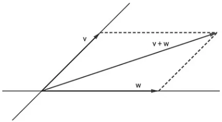
Fig. 1.1 The parallelogram rule

IfS_{denotes the usual three dimensional physical space, we denote by} W3= {B−A| A,B∈S}

the collection of all applied vectors at any point ofS_{and by} V3

A = {B−A| B∈S} the collection of all vectors applied atAinS_{. Then}

W3= A∈S

V3_A.

Remark 1.1.1 Once fixed a pointOinS_{, one sees that there is a bijection between} the set V3

O= {B−O | B∈S}andS itself. Indeed, each point B inS uniquely determines the element B−O inV3

O, and each element B−O inV 3

O uniquely determines the pointBinS_.

It is well known that the so called parallelogram ruledefines inV3

O a sum of vectors, where

(A−O)+(B−O)=(C−O),

withC the fourth vertex of the parallelogram whose other three vertices are A,O, B, as shown in Fig.1.1.

The vector0=O−Ois called thezero vector(ornull vector); notice that its modulus is zero, while its direction and orientation are undefined.

It is evident thatV3

O is closed with respect to the notion of sum defined above. That such a sum is associative and abelian is part of the content of the proposition that follows.

Proposition 1.1.2 The datum(V3

O,+,0)is an abelian group.

(14)

1.1 Applied Vectors 3

Fig. 1.2 The opposite of a vector:A′−O= −(A−O)

Fig. 1.3 The associativity of the vector sum

with respect to the sum (that is, any vector has an opposite vector) given byA′₋_O, where A′_{is the symmetric point to}_A_{with respect to}_O_{on the straight line joining}

AtoO(see Fig.1.2).

From its definition the sum of two vectors is a commutative operation. For the associativity we give a pictorial argument in Fig.1.3. There is indeed more structure. The physical intuition allows one to consider multiples of an applied vector. Concerning the collectionV3

O, this amounts to define an operation involving vectors applied inOand real numbers, which, in order not to create confusion with vectors, are called (real)scalars.

Definition 1.1.3 Given the scalarλ∈ _Rand the vectorA−O ∈ V3

O, theproduct by a scalar

B − O = λ(A − O) is the vector such that:

(i) A,B,Oare on the same (straight) line,

(ii) B − O and A − O have the same orientation if λ>0, while A − O and B − Ohave opposite orientations ifλ<0,

(iii) B − O = |λ| A − O.

The main properties of the operation of product by a scalar are given in the following proposition.

Proposition 1.1.4 For any pair of scalars λ,µ ∈ _R and any pair of vectors A − O, B − O ∈ V3

(15)

Fig. 1.4 The scalingλ(C−O)=(C′−O)withλ>1

1. λ(µ(A − O)) = (λµ)(A − O), 2. 1(A − O) = A − O,

3. λ((A − O)+(B − O)) = λ(A − O) +λ(B − O), 4. (λ+µ)(A − O) = λ(A − O)+µ(A − O).

Proof 1. SetC − O = λ(µ(A − O))andD − O = (λµ)(A − O). If one of the scalarsλ,µ is zero, one trivially has C − O = 0 and D − O = 0, so Point 1.is satisfied. Assume now thatλ=0 and µ=0. Since, by definition, bothCandDare points on the line determined byOandA, the vectorsC − O andD − Ohave the same direction. It is easy to see thatC − OandD − O have the same orientation: it will coincide with the orientation ofA − Oor not, depending on the sign of the productλµ=0. Since|λµ| = |λ||µ| ∈ R, one has

C − O = D − O.

2. It follows directly from the definition.

3. SetC − O = (A − O)+(B − O)andC′ − O = (A′ − O)+(B′ − O), withA′ − O = λ(A − O)andB′ − O = λ(B − O).

We verify thatλ(C − O) = C′ ₋ _O_{(see Fig.}_1.4).

SinceO Ais parallel toO A′_{by definition, then} _BC _{is parallel to}_B′_C′_;_{O B} _is indeed parallel to O B′, so that the planar anglesO BC andO B′_C′ _{are equal.} Alsoλ(O B) = O B′_,_{λ(O A)} ₌ _{O A}′_{, and}_λ(BC₎ ₌ _B′_C′_{. It follows that the} trianglesO BCandO B′_C′_{are similar: the vector}_OC_{is then parallel} _OC′_and they have the same orientation, withOC′₌_λ_{OC. From this we obtain} OC′ ₌ _λ(OC).

4. The proof is analogue to the one in point 3.

What we have described above shows that the operations of sum and product by a scalar giveV3

(16)

1.2 Coordinate Systems 5

1.2 Coordinate Systems

The notion of coordinate system is well known. We rephrase its main aspects in terms of vector properties.

Definition 1.2.1 Given a liner, acoordinate systemon it is defined by a point O ∈ rand a vectori = A − O, where A∈r andA=O.

The pointOis called theoriginof the coordinate system, the normA − Ois theunit of measure(orlength)of, withithe basisunit vector. The orientation of iis theorientationof the coordinate system.

A coordinate systemprovides a bijection between the points on the linerand

R. Any pointP∈rsingles out the real numberxsuch thatP − O = xi; viceversa, for anyx ∈_Rone has the point P∈rdefined by P − O = xi. One says thatP has coordinatex, and we shall denote it byP=(x), with respect to the coordinate systemthat is also denoted as(O;x)or(O;i).

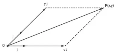
Definition 1.2.2 Given a planeα, a coordinate systemon it is defined by a point O ∈ αand a pair of non zero distinct (and not having the same direction) vectors i = A − Oandj = B − OwithA,B ∈ α, andA − O = B − O.

The point Ois the origin of the coordinate system, the (common) norm of the vectors i,j is the unit length of, withi,jthe basis unit vectors. The system is oriented in such a way that the vector i coincides with j after an anticlockwise rotation of angle φwith 0<φ<π. The line defined by O andi, with its given orientation, is usually referred to as a theabscissa axis, while the one defined byO andj, again with its given orientation, is calledordinate axis.

As before, it is immediate to see that a coordinate systemonαallows one to define a bijection between points on α andordered pairs of real numbers. Any P ∈ α uniquely provides, via the parallelogram rule (see Fig.1.5), the ordered pair (x,y)∈_R2 _with _P ₋ _O ₌ _xi ₊ _{yj; conversely, for any given ordered pair} (x,y)∈_R2_{, one defines}_P _∈ _α_{as given by}_P ₋ _O ₌ _xi ₊ _yj.

With respect to, the elementsx ∈ _Rand y ∈ _Rare thecoordinates of P, and this will be denoted by P=(x,y). The coordinate systemwill be denoted (O;i,j)or(O;x,y).

(17)

Definition 1.2.3 A coordinate system=(O;i,j)on a planeαis called an orthog-onal cartesian coordinate systemifφ=π/2, whereφis as before the width of the anticlockwise rotation under whichicoincides withj.

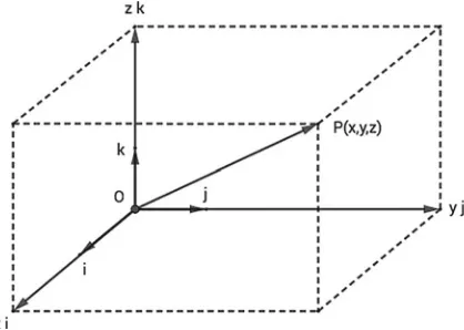
In order to introduce a coordinate system for the physical three dimensional space, we start by considering three unit-length vectors inV3

Ogiven asu = U − O, v = V − O,w = W − O, and we assume the pointsO,U,V,Wnot to be on the same plane. This means that any two vectors,uandvsay, determine a plane which does not contain the third point, sayW. Seen fromW, the vectoruwill coincide withvunder an anticlockwise rotation by an angle that we denote byuv.

Definition 1.2.4 An ordered triple(u,v,w)of unit vectors inV3

Owhich do not lie on the same plane is calledright-handedif the three anglesuv, vw, wu, defined by the prescription above are smaller thanπ. Notice that the order of the vectors matters. Definition 1.2.5 A coordinate systemfor the spaceS_{is given by a point}O ∈ S and three non zero distinct (and not lying on the same plane) vectorsi = A − O, j = B − Oandk = C − O, withA,B,C ∈ S_{, and}A − O = B − O = C − Oand(i,j,k)giving a right-handed triple.

The point O is theoriginof the coordinate system, the common length of the vectorsi,j,kis the unit measure in, withi,j,k the basisunit vectors. The line defined byOandi, with its orientation, is the abscissa axis, that defined byOandj is the ordinate axis, while the one defined byOandkis the quota axis.

With respect to the coordinate system , one establishes, via V3

O, a bijection between ordered triples of real numbers and points inS_{. One has}

P ↔ P − O ↔ (x,y,z)

withP − O = xi+yj+zkas in Fig.1.6. The real numbersx,y,zare the com-ponents(orcoordinates) of the applied vectorP − O, and this will be denoted by P=(x,y,z). Accordingly, the coordinate system will be denoted by = (O;i,j,k) = (O;x,y,z). The coordinate systemis called cartesian orthog-onal if the vectorsi,j,kare pairwise orthogonal.

By writingv = P − O, it is convenient to denote byvx,vy,vzthe components ofvwith respect to a cartesian coordinate system, so to have

v=vxi+vyj+vzk. In order to simplify the notations, we shall also write this as

v=(vx,vy,vz),

(18)

Fig. 1.6 The bijectionP(x,y,z)↔ P−O=xi+yj+zkin the space

Exercise 1.2.6 One has

1. The zero (null) vector0 = O − Ohas components(0,0,0)with respect to any coordinate system whose origin isO, and it is the only vector with this property. 2. Given a coordinate system = (O;i,j,k), the basis unit vectors have

compo-nents

i=(1,0,0) , j=(0,1,0) , k=(0,0,1).

3. Given a coordinate system = (O;i,j,k)for the spaceS_{, we call}_coordinate planeeach plane determined by a pair of axes of. We havev=(a,b,0), with a,b∈_R, ifvis on the plane x y,v′₌_(0,_b′_,_c′₎_if_v′_{is on the plane} _{yz, and} v′′₌_(a′′_,_0,_c′′₎_if_v′′_{is on the plane}_{x z.}

Example 1.2.7 The motion of a point mass in three dimensional space is described by a mapt∈_R → x(t)∈V3

Owheretrepresents thetimevariable andx(t) is the posi-tion of the point mass at timet. With respect to a coordinate system =(O;x,y,z) we then write

x(t) = (x(t),y(t),z(t)) or equivalently x(t) = x(t)i+y(t)j+z(t)k. The corresponding velocity is a vector applied in x(t), that is v(t)∈V3

x(t), with components

v(t) = (vx(t),vy(t),vz(t)) = dx(t)

dt = ( dx dt ,

dy dt ,

dz dt), while the acceleration is the vectora(t)∈V3

x(t)with components

a(t) = dv(t) dt = (

dx2 dt2 ,

d2_y dt2 ,

(19)

One also uses the notations

v=dx

dt = ˙x and a= d2x

dt2 = ˙v= ¨x.

In the newtonian formalism for the dynamics, aforceacting on the given point mass is a vector applied inx(t), that isF∈V_x3_(t)_{with components}F=(Fx,Fy,Fz), and thesecond law of dynamicsis written as

ma = F

where m>0 is the value of theinertial mass of the moving point mass. Such a relation can be written component-wise as

md 2_x

dt2 = Fx, m d2_y

dt2 = Fy, m d2_z dt2 = Fz.

A coordinate system forS_{allows one to express the operations of sum and product} by a scalar inV3

Oin terms of elementary algebraic expressions.

Proposition 1.2.8 With respect to the coordinate system = (O;i,j,k), let us consider the vectorsv=vxi+vyj+vzkandw=wxi+wyj+wzk, and the scalar λ ∈ _R. One has:

(1) v+w=(vx+wx)i+(vy+wy)j+(vz+wz)k, (2) λv=λvxi+λvyj+λvzk.

Proof (1) Sincev+w=(vxi+vyj+vzk)+(wxi+wyj+wzk), by using the com-mutativity and the associativity of the sum of vectors applied at a point, one has

v+w=(vxi+wxi)+(vyj+wyj)+(vzk+wzk).

Being the product distributive over the sum, this can be regrouped as in the claimed identity.

(2) Along the same lines as (1).

Remark 1.2.9 By denoting v=(vx,vy,vz) and w=(wx, wy, wz), the identities proven in the proposition above are written as

(vx,vy,vz)+(wx, wy, wz)=(vx+wx,vy+wy,vz+wz), λ(vx,vy,vz)=(λvx,λvy,λvz).

This suggests a generalisation we shall study in detail in the next chapter. If we denote byR3

(20)

elements(x1,x2,x3)and(y1,y2,y3)inR3, withλ∈R, one can introduce a sum of triples and a product by a scalar:

(x1,x2,x3)+(y1,y2,y3)=(x1+y1,x2+y2,x3+y3), λ(x1,x2,x3)=(λx1,λx2,λx3).

1.3 More Vector Operations

In this section we recall the notions—originating in physics—of scalar product, vector product and mixed products.

Before we do this, as an elementary consequence of the Pythagora’s theorem, one has the following (see Fig.1.6)

Proposition 1.3.1 Letv = (vx,vy,vz)be an arbitrary vector inV3

Owith respect to the cartesian orthogonal coordinate system(O;i,j,z). One has

v =

v2

x+v2y+vz2. Definition 1.3.2 Let us consider a pair of vectorsv,w∈V3

O. Thescalar productof vandw, denoted byv·w, is the real number

v·w= v wcosα

withα=vw the plane angle defined byvandw. Since cosα=cos(−α), for this definition one has cosvw = coswv.

The definition of a scalar product for vectors inV2_O_{is completely analogue.} Remark 1.3.3 The following properties follow directly from the definition. (1) Ifv = 0, thenv·w=0.

(2) Ifv,ware both non zero vectors, then

v·w=0 ⇐⇒ cosα=0 ⇐⇒ v⊥w. (3) For anyv∈V3

O, it holds that:

v·v= v2 and moreover

(21)

(4) From(2), (3), if(O;i,j,k)is an orthogonal cartesian coordinate system, then i·i=j·j=k·k=1, i·j=j·k=k·i=0.

Proposition 1.3.4 For any choice ofu,v,w∈V3

Oandλ∈R, the following identi-ties hold.

(i) v·w=w·v,

(ii) (λv)·w=v·(λw)=λ(v·w), (iii) u·(v+w)=u·v+u·w.

Proof (i) From the definition one has

v·w= v wcosvw= w vcoswv =w·v.

(ii) Settinga=(λv)·w,b=v·(λw)andc=λ(v·w), from the Definition1.3.2 and the properties of the norm of a vector, one has

a=(λv)·w= λv wcosα′= |λ|v wcosα′ b=v·(λw)= v λwcosα′′= v |λ|wcosα′′ c=λ(v·w)=λ(v wcosα)=λv wcosα

whereα′₌_(λv)w, _α′′₌_v(λw) _and_α₌_{vw. If} _λ₌_{0, then}_a₌_b₌_c₌_0. If λ>0, then |λ| =λ and α=α′₌_α′′_{; from the commutativity and the} associativity of the product in R, this gives that a=b=c. If λ<0, then |λ| = −λandα′₌_α′′₌_π₋_{α, thus giving cos}_α′₌_cos_α′′_{= −}_cos_{α. These} reada=b=c.

(iii) We sketch the proof for parallelu,v,w. Under this condition, the result depends on the relative orientations of the vectors. Ifu,v,whave the same orientation, one has

u·(v+w)= u v+w = u(v + w) = u v + u w =u·v+u·w.

Ifvandwhave the same orientation, which is not the orientation ofu, one has u·(v+w)= −u v+w

= −u(v + w) = −u v − u w =u·v+u·w.

(22)

1.3 More Vector Operations 11

By expressing vectors inV3_O_{in terms of an orthogonal cartesian coordinate system,} the scalar product has an expression that will allow us to define the scalar product of vectors in the more general situation of euclidean spaces.

Proposition 1.3.5 Given(O;i,j,k), an orthogonal cartesian coordinate system for S; with vectorsv=(vx,vy,vz)andw=(wx, wy, wz)inV3

O, one has v·w=vxwx+vywy+vzwz.

Proof Withv=vxi+vyj+vzkandw=wxi+wyj+wzk, from Proposition1.3.4, one has

v·w= (vxi+vyj+vzk)·(wxi+wyj+wzk) = vxwxi·i+vywxj·i+vzwxk·i

+ vxwyi·j+vywyj·j+vzwyk·j+ vxwzi·k+vywzj·k+vzwzk·k. The result follows directly from (4) in Remark1.3.3, that isi·j=j·k=k·i=0

as well asi·i=j·j=k·k=1.

Exercise 1.3.6 With respect to a given cartesian orthogonal coordinate system, con-sider the vectorsv=(2,3,1)andw=(1,−1,1). We verify they are orthogonal. From (2) in Remark1.3.3this is equivalent to show thatv·w=0. From Proposition 1.3.5, one hasv·w=2·1+3·(−1)+1·1=0.

Example 1.3.7 If the mapx(t):_R ∋ t → x(t)∈V3

Odescribes the motion (notice that the range of the map gives the trajectory) of a point mass (with massm), its kinetic energyis defined by

T = 1

2mv(t) 2

.

With respect to an orthogonal coordinate system =(O;i,j,k), given v(t)=(vx(t),vy(t),vz(t)) as in the Example 1.2.7, we have from the Proposi-tion1.3.5that

T = 1 2m(v

2 x+v

2 y+v

2 z).

Also the following notion will be generalised in the context of euclidean spaces. Definition 1.3.8 Given two non zero vectorsvandwinV3

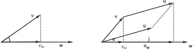
O, theorthogonal projec-tionofvalongwis defined as the vectorvwinVO3 given by

vw= v·w w2w. As the first part of Fig.1.7displays,vwis parallel tow.

(23)

Fig. 1.7 Orthogonal projections

Proposition 1.3.9 For anyu,v,w∈V3

O, the following identities hold: (a) (u+v)w=uw+vw,

(b) v·w=vw·w=wv·v.

The point(a)is illustrated by the second part of the Fig.1.7. Remark 1.3.10 The scalar product we have defined is a map

σ:V3 O×V

3

O−→R, σ(v,w)=v·w. Also, the scalar product of vectors on a plane is a mapσ:V2

O×V 2

O−→R. Definition 1.3.11 Letv,w∈V3

O. Thevector productbetweenvandw, denoted by v∧w, is defined as the vector inV3

Owhose modulus is v∧w = v wsinα,

whereα=vw, with 0 <α<πis the angle defined byvew; the direction ofv∧w is orthogonal to both v andw; and its orientation is such that (v,w,v∧w)is a right-handed triple as in Definition1.2.4.

Remark 1.3.12 The following properties follow directly from the definition. (i) ifv=0thenv∧w=0,

(ii) ifvandware both non zero then

v∧w=0 ⇐⇒ sinα=0 ⇐⇒ vw, (one trivially hasv∧v=0),

(iii) if(O;i,j,k)is an orthogonal cartesian coordinate system, then

(24)

1.3 More Vector Operations 13

Proposition 1.3.13 For anyu,v,w∈V3_Oandλ∈R, the following identities holds: (i) v∧w= −w∧v,

(ii) (λv)∧w=v∧(λw)=λ(v∧w) (iii) u∧(v+w)=u∧v+u∧w,

Exercise 1.3.14 With respect to a given cartesian orthogonal coordinate system, consider inV3_O_{the vectors}v=(1,0,−1)ew=(−2,0,2). To verify that they are parallel, we recall the abov e result (ii) in the Remark1.3.12and compute, using the Proposition1.3.15, thatv∧w=0.

Proposition 1.3.15 Letv=(vx,vy,vz)and w=(wx, wy, wz)be elements inV3_O with respect to a given cartesian orthogonal coordinate system. It is

v∧w=(vywz−vzwy,vzwx−vxwz,vxwy−vywx).

Proof Given the Remark1.3.12and the Proposition1.3.13, this comes as an easy

computation.

Remark 1.3.16 The vector product defines a map τ :V3

O×V 3 O−→V

3

O, τ(v,w)=v∧w. Clearly, such a map has no meaning on a plane.

Example 1.3.17 By slightly extending the Definition1.3.11, one can use the vec-tor product for additional notions coming from physics. Following Sect.1.1, we consider vectors u,w as elements in W3_{, that is vectors applied at arbitrary} points in the physical three dimensional spaceS_{, with components}u=(ux,uy,uz) and w=(wx, wy, wz) with respect to a cartesian orthogonal coordinate system =(O;i,j,k). In parallel with Proposition1.3.15, we defineτ : W3_×_W3 _→ _W3 as

u∧w = (uywz−uzwy,uzwx−uxwz,uxwy−uywx).

Ifu∈V_x3_{is a vector applied at}_{x, its}momentumwith respect to a pointx′∈S_{is the} vector inW3

defined by

M = (x−x′)∧u.

In particular, ifu=F is a force acting on a point mass inx, its momentum is M = (x−x′₎_∧_F.

If x(t)∈V3

O describes the motion of a point mass (with massm>0), whose velocity isv(t), then its correspondingangular momentumwith respect to a pointx′ is defined by

(25)

Exercise 1.3.18 The angular momentum is usually defined with respect to the origin of the coordinate system, givingLO(t) = x(t)∧ mv(t). If we consider a circular uniform motion

x(t)=x(t)=rcos(ωt), y(t)=rsin(ωt), z(t)=0

,

withr >0 the radius of the trajectory andω∈_Rthe angular velocity, then

v(t)=

vx(t)= −rωsin(ωt), y(t)=rωcos(ωt), vz(t)=0

so that

LO(t) = (0,0,mrω).

Thus, a circular motion on thex yplane has angular momentum along thezaxis. Definition 1.3.19 Given anorderedtripleu,v,w∈V3

O, theirmixed productis the real number

u·(v∧w).

Proposition 1.3.20 Given a cartesian orthogonal coordinate system in S with u=(ux,uy,uz),v=(vx,vy,vz)andw=(wx, wy, wz)inV3_O, one has

u·(v∧w)=ux(vywz−vzwy)+uy(vzwx−vxwz)+uz(vxwy−vywx). Proof It follows immediately by Propositions1.3.5and1.3.15.

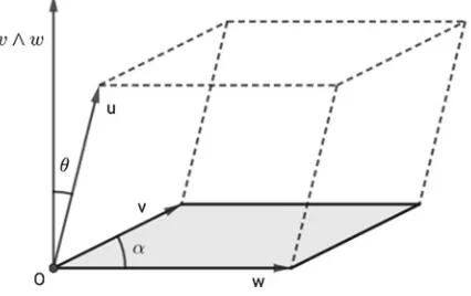
In the spaceS_{, the vector product between}u∧wis the area of the parallelogram defined by u and v, while the mixed product u·(v∧w)give the volume of the parallelepiped defined byu,v,w.

Proposition 1.3.21 Givenu,v,w∈V3 O.

1. Denoteα=vwthe angle defined byvandw. Then, the area A of the parallelo-gram whose edges areuandv, is given by

A= v wsinα= v∧w.

2. Denoteθ=u(v∧w)the angle defined byuandv∧w. Then the volume V of the parallelepiped whose edges areu,v,w, is given by

V =Aucosθ= u·v∧w.

(26)

1.4 Divergence, Rotor, Gradient and Laplacian 15

Fig. 1.8 The area of the parallelogramm with edgesvandw

Fig. 1.9 The volume of the parallelogramm with edgesv,w,u

1.4 Divergence, Rotor, Gradient and Laplacian

We close this chapter by describing how the notion of vector applied at a point also allows one to introduce a definition of avector field.

The intuition coming from physics requires to consider, for each pointxin the physical spaceS_{, a vector applied at}_{x. We describe it as a map}

S ∋ x → A(x) ∈ V_x3.

With respect to a given cartesian orthogonal reference system forS _{we can write} this in components asx=(x1,x2,x3)andA(x)=(A1(x),A2(x),A3(x))and one can act on a vector field with partial derivatives (first order differential operators), ∂a =(∂/∂xa)witha =1,2,3, defined as usual by

∂a(xb)=(δab), with δab=

1 if a =b 0 if a=b . Then, (omitting the explicit dependence ofAonx) one defines

divA = 3

k=1

(∂kAk)∈R

(27)

By introducing the triple∇ =(∂1,∂2,∂3), such actions can be formally written as a scalar product and a vector product, that is

divA = ∇ ·A rotA = ∇ ∧A.

Furthermore, if f :S→_Ris a real valued function defined onS_{, that is a (real)} scalar fieldonS_{, one has the grad operator}

grad f = ∇f = (∂1f,∂2f,∂3f) as well as the Laplacian operator

∇2 f = div(∇f)= 3

k=1

∂k∂kf = ∂2 1f +∂

2 2 f +∂

2 3f .

Exercise 1.4.1 The properties of the mixed products yields a straightforward proof of the identity

div(rotA) = ∇ ·(∇ ∧A) = 0,

for any vector fieldA. On the other hand, a direct computation shows also the identity rot(grad f)= ∇ ∧(gradf) = 0,

(28)

Chapter 2 Vector Spaces

The notion of vector space can be defined over any fieldK_{. We shall mainly consider} the caseK = R_{and briefly mention the case}K = C_{. Starting from our exposition,} it is straightforward to generalise to any field.

2.1 Definition and Basic Properties

The model of the construction is the collection of all vectors in the space applied at a point with the operations of sum and multiplication by a scalar, as described in the Chap.1.

Definition 2.1.1 A non empty setVis called avector space overR_{(or a}real vector spaceor anR_{-vector space) if there are defined two operations,}

(a) an internal one: a sum of vectorss : V ×V → V,

V ×V ∋(v, v′)→s(v, v′)=v+v′,

(b) an exterior one: the product by a scalar p:R_×_V _→_V

R_×_V _∋_{(k, v)}_→_{p(k, v)}₌_kv,

and these operations are required to satisfy the following conditions:

(1) There exists an element 0V ∈V, which is neutral for the sum, such that

(V,+,0V)is an abelian group.

For anyk,k′_∈_R_and_{v, v}′_∈_V _{one has} (2) (k+k′_)v₌_kv₊_k′_v

(3) k(v+v′₎₌_kv₊_kv′

© Springer International Publishing AG, part of Springer Nature 2018 G. Landi and A. Zampini,Linear Algebra and Analytic Geometry for Physical Sciences, Undergraduate Lecture Notes in Physics, https://doi.org/10.1007/978-3-319-78361-1_2

(29)

18 2 Vector Spaces

(4) k(k′_v)₌_(kk′_)v (5) 1v=v, with 1=1R.

The elements of a vector space are calledvectors; the element 0V is thezeroornull

vector. A vector space is also called alinear space.

Remark 2.1.2 Given the properties of a group (see A.2.9), the null vector 0V and the

opposite−vto any vectorvare (in any given vector space) unique. The sums can be indeed simplified, that isv+w=v+u =⇒w=u. Such a statement is easily proven by adding to both terms in v+w=v+u the element−v and using the associativity of the sum.

As already seen in Chap.1, the collectionsV2_O_{(vectors in a plane) and}V3

O(vectors

in the space) applied at the pointOare real vector spaces. The bijectionV3

O ←→R3

introduced in the Definition1.2.5, together with the Remark1.2.9, suggest the natural definitions of sum and product by a scalar for the setR3 _{of ordered triples of real} numbers.

Proposition 2.1.3 The collectionR3 _{of triples of real numbers together with the} operations defined by

I. (x1,x2,x3)+(y1,y2,y3)=(x1+y1,x2+y2,x3+y3), for any (x1,x2,x3), (y1,y2,y3)∈R3_,

II. a(x1,x2,x3)=(ax1,ax2,ax3), for any a∈R,(x1,x2,x3)∈R3_,

is a real vector space.

Proof We verify that the conditions given in the Definition2.1.1are satisfied. We first notice that (a)and (b)are fullfilled, since R3 _{is closed with respect to the} operations in I. and II. of sum and product by a scalar. The neutral element for the sum is 0R3=(0,0,0), since one clearly has

(x1,x2,x3)+(0,0,0)=(x1,x2,x3).

The datum(R3,+,0R3)is an abelian group, since one has

• The sum(R3_,₊₎

is associative, from the associativity of the sum inR_:

(x1,x2,x3)+((y1,y2,y3)+(z1,z2,z3))

(30)

2.1 Definition and Basic Properties 19

• From the identity

(x1,x2,x3)+(−x1,−x2,−x3)=(x1−x1,x2−x2,x3−x3)=(0,0,0)

one has(−x1,−x2,−x3)as the opposite inR3

of the element(x1,x2,x3). • The group(R3_,₊₎

is commutative, since the sum inR_{is commutative:}

(x1,x2,x3)+(y1,y2,y3)=(x1+y1,x2+y2,x3+y3) =(y1+x1,y2+x2,y3+x3) =(y1,y2,y3)+(x1,x2,x3).

We leave to the reader the task to show that the conditions(1), (2), (3), (4)in Defi-nition2.1.1are satisfied: for anyλ,λ′_∈_R_{and any}_(x1,_x2,_x3),_(y1,_y2,_y3)_∈_R3_it holds that

1. (λ+λ′_)(x1,_x2,_x3)₌_λ(x1,_x2,_x3)₊_λ′_(x1,_x2,_x3)

2. λ((x1,x2,x3)+(y1,y2,y3))=λ(x1,x2,x3)+λ(y1,y2,y3) 3. λ(λ′_(x1,_x2,_x3))₌_(λλ′_)(x1,_x2,_x3)

4. 1(x1,x2,x3)=(x1,x2,x3).

The previous proposition can be generalised in a natural way. Ifn∈N_{is a positive} natural number, one defines then-th cartesian product ofR_{, that is the collection of} orderedn-tuples of real numbers

Rn= {X =(x1, . . . ,xn) : xk∈R},

and the following operations, witha∈R_,(x1, . . . ,xn),(y1, . . . ,yn)∈Rn:

In. (x1, . . . ,xn)+(y1, . . . ,yn)=(x1+y1, . . . ,xn+yn)

IIn. a(x1, . . . ,xn)=(ax1, . . . ,axn).

The previous proposition can be directly generalised to the following.

Proposition 2.1.4 With respect to the above operations, the setRn_{is a vector space}

overR_.

The elements in Rn _{are called} _n-tuples _{of real numbers. With the notation}

X=(x1, . . . ,xn)∈Rn, the scalar xk, withk=1,2, . . . ,n, is thek-th component

of the vector X.

Example 2.1.5 As in the Definition A.3.3, consider the collection of all polynomials in the indeterminatexand coefficients inR_{, that is}

R[x] =

f(x)=a0+a1x+a2x2+ · · · +anxn : ak∈R,n≥0

,

with the operations of sum and product by a scalarλ∈R_{defined, for any pair of} elements in R[x], f(x)=a0+a1x+a2x2_{+ · · · +}_a

nxn and g(x)=b0+b1x+

b2x2_{+ · · · +}_b

(31)

20 2 Vector Spaces

Ip. f(x)+g(x)=a0+b0+(a1+b1)x+(a2+b2)x2_{+ · · ·} IIp. λf(x)=λa0+λa1x+λa2x2+ · · · +λanxn.

Endowed with the previous operations, the setR_[x]is a real vector space;R_[x]is indeed closed with respect to the operations above. The null polynomial, denoted by 0R[x](that is the polynomial with all coefficients equal zero), is the neutral element for the sum. The opposite to the polynomial f(x)=a0+a1x+a2x2+ · · · +anxn

is the polynomial (−a0−a1x−a2x2_{− · · · −}_a

nxn) ∈ R[x]that one denotes by −f(x). We leave to the reader to prove that(R[x],+,0R[x])is an abelian group and that all the additional conditions in Definition2.1.1are fulfilled.

Exercise 2.1.6 We know from the Proposition A.3.5 thatR[x]r, the subset inR[x]

of polynomials with degree not larger than a fixedr ∈ N_{, is closed under addition} of polynomials. Since the degree of the polynomialλf(x)coincides with the degree of f(x)for anyλ=0, we see that also the product by a scalar, as defined in IIp. above, is defined consistently onR[x]r. It is easy to verify that alsoR[x]r is a real

vector space.

Remark 2.1.7 The proof thatRn_,_R_[_x_]_and_R_[_x_]

rare vector space overRrelies on

the properties ofR_{as a field (in fact a ring, since the multiplicative inverse in}R_does not play any role).

Exercise 2.1.8 The setCn_{, that is the collection of ordered}_n_{-tuples of complex}

numbers, can be given the structure of a vector space over C_{. Indeed, both the} operations In. and IIn. considered in the Proposition2.1.3when intended for complex numbers make perfectly sense:

Ic. (z1, . . . ,zn)+(w1, . . . , wn)=(z1+w1, . . . ,zn+wn)

IIc. c(z1, . . . ,zn)=(cz1, . . . ,czn)

withc∈C_{, and}(z1, . . . ,zn),(w1, . . . , wn)∈Cn.

The reader is left to show thatCn_{is a vector space over}_C_.

The spaceCn _{can also be given a structure of vector space over}_R_{, by noticing}

that the product of a complex number by a real number is a complex number. This means thatCn

is closed with respect to the operations of (component-wise) product by a real scalar. The condition IIc. above makes sense whenc∈R_.

We next analyse some elementary properties of general vector spaces.

Proposition 2.1.9 Let V be a vector space overR_{. For any k}_∈R_{and any}_v_∈_{V it} holds that:

(i) 0Rv=0V,

(ii) k0V =0V,

(iii) if kv=0V then it is either k=0Rorv=0V,

(iv) (−k)v= −(kv)=k(−v).

Proof (i) From 0Rv=(0R+0R)v=0Rv+0Rv, since the sums can be simpli-fied, one has that 0Rv=0V.

(32)

2.1 Definition and Basic Properties 21

(iii) Letk=0, sok−1 _∈_R_{exists. Then,}_v₌_1v₌_k−1_kv₌_k−1₀

V =0V, with the

last equality coming from (ii).

(iv) Since the product is distributive over the sum, from (i) it follows that kv+(−k)v=(k+(−k))v=0Rv=0V that is the first equality. For the

sec-ond, one writes analogouslykv+k(−v)=k(v−v)=k0V =0V

Relations (i), (ii), (iii) above are more succinctly expressed by the equivalence:

kv=0V ⇐⇒k=0R or v=0V.

2.2 Vector Subspaces

Among the subsets of a real vector space, of particular relevance are those which inherit fromV a vector space structure.

Definition 2.2.1 LetV be a vector space overR_{with respect to the sum}_s_{and the} product pas given in the Definition2.1.1. LetW ⊆V be a subset ofV. One says thatW is avector subspaceofV if the restrictions ofsandp toW equipW with the structure of a vector space overR_.

In order to establish whether a subsetW ⊆V of a vector space is a vector subspace, the following can be seen ascriteria.

Proposition 2.2.2 Let W be a non empty subset of the real vector space V . The following conditions are equivalent.

(i) W is a vector subspace of V ,

(ii) W is closed with respect to the sum and the product by a scalar, that is

(a) w+w′_∈_{W ,} _{for any}_{w, w}′_∈_{W ,} (b) kw∈W , for any k∈Randw∈W ,

(iii) kw+k′_w′_∈_{W ,} _{for any k,}_k′_∈_R_{and any}_{w, w}′_∈_{W .}

Proof The implications(i)=⇒ii)and(ii)=⇒(iii)are obvious from the definition.

(iii)=⇒(ii): By takingk=k′=1 one obtains (a), while to show point (b) one takesk′=0R.

(ii)=⇒(i): Notice that, by hypothesis,W is closed with respect to the sum and product by a scalar. Associativity and commutativity hold inW since they hold inV. One only needs to prove thatW has a neutral element 0W and that, for such a

neutral element, any vector inW has an opposite inW. If 0V ∈W, then 0V is the

zero element inW: for anyw∈W one has 0V +w=w+0V =wsincew∈V;

from ii, (b) one has 0Rw∈W for anyw∈W; from the Proposition2.1.9one has 0Rw=0V; collecting these relations, one concludes that 0V ∈W. Ifw∈W, again

(33)

22 2 Vector Spaces

Exercise 2.2.3 BothW = {0V} ⊂V andW =V ⊆V aretrivialvector subspaces

ofV.

Exercise 2.2.4 We have already seen that R[x]r ⊆R[x] are vector spaces with

respect to the same operations, so we may conclude thatR[x]r is a vector subspace

ofR[x].

Exercise 2.2.5 Letv∈V a non zero vector in a vector space, and let

L(v)= {av : a ∈R} ⊂V

be the collection of all multiples ofvby a real scalar. Given the elementsw=av andw′₌_a′_v_in_L_{(v), from the equality}

αw+α′w′=(αa+α′a′)v∈L(v)

for anyα,α′_∈_R_{, we see that, from the Proposition}_2.2.2,_L_(v)_{is a vector subspace} ofV, and we call it the (vector)line generated byv.

Exercise 2.2.6 Consider the following subsetsW ⊂ R2_:

1. W1= {(x,y)∈R2 _: _x₋₃_y₌₀_}_, 2. W2= {(x,y)∈R2 _: _x₊_y₌₁_}_, 3. W3= {(x,y)∈R2 _: _x_∈_N_}_, 4. W4= {(x,y)∈R2 : x2−y=0}.

From the previous exercise, one sees that W1 is a vector subspace since W1=L_((3,_{1)). On the other hand,}_W2,_W3,_W4_{are not vector subspaces of}R2

. The zero vector(0,0) /∈W2; whileW3andW4are not closed with respect to the product by a scalar, since, for example,(1,0)∈W3but1₂(1,0)=(1₂,0) /∈W3. Analogously, (1,1)∈W4but 2(1,1)=(2,2) /∈W4.

The next step consists in showing how, given two or more vector subspaces of a real vector spaceV, one can define new vector subspaces ofVvia suitable operations.

Proposition 2.2.7 The intersection W1∩W2of any two vector subspaces W1and W2of a real vector space V is a vector subspace of V .

Proof Considera,b∈R_and_{v, w}_∈_W1_∩_{W2. From the Propostion}_2.2.2_{it follows} thatav+bw∈W1sinceW1is a vector subspace, and also thatav+bw∈W2for the same reason. As a consequence, one hasav+bw∈W1∩W2.

Remark 2.2.8 In general, the union of two vector subspaces of V isnot a vector subspace ofV. As an example, the Fig.2.1shows that, ifL_(v)_andL_(w)_{are generated} by differentv, w ∈ R2

(34)

2.2 Vector Subspaces 23

Fig. 2.1 The vector lineL(v+w)with respect to the vector linesL(v)andL(w)

Proposition 2.2.9 Let W1and W2 be vector subspaces of the real vector space V and let W1+W2denote

W1+W2= {v∈V |v=w1+w2; w1∈W1, w2 ∈W2} ⊂V.

Then W1+W2 is the smallest vector subspace of V which contains the union W1∪W2.

Proof Leta,a′∈R_and_{v, v}′_∈_W1₊

W2; this means that there existw1, w₁′ ∈W1 andw2, w′₂∈W2, so thatv=w1+w2andv′=w′₁+w₂′. Since bothW1 andW2 are vector subspaces ofV, from the identity

av+a′v′=aw1+aw2+a′w₁′ +a′w₂′ =(aw1+a′w′₁)+(aw2+a′w₂′),

one hasaw1+a′w′1∈W1andaw2+a′w2′ ∈W2. It follows thatW1+W2is a vector subspace ofV.

It holds that W1+W2⊇W1∪W2: if w1∈W1, it is indeedw1=w1+0V in

W1+W2; one similarly shows thatW2⊂W1+W2.

Finally, let Z be a vector subspace of V containing W1∪W2; then for any w1∈W1 andw2 ∈W2 it must bew1+w2∈Z. This implies Z ⊇W1+W2, and thenW1+W2is the smallest of such vector subspacesZ.

Definition 2.2.10 IfW1andW2are vector subspaces of the real vector spaceV the vector subspaceW1+W2ofV is called thesumofW1eW2.

The previous proposition and definition are easily generalised, in particular:

Definition 2.2.11 IfW1, . . . ,Wn are vector subspaces of the real subspace V, the

vector subspace

W1+ · · · +Wn = {v∈V |v=w1+ · · · +wn; wi ∈Wi, i=1, . . . ,n}

(35)

24 2 Vector Spaces

Definition 2.2.12 LetW1andW2be vector subspaces of the real vector spaceV. The sumW1+W2is calleddirectifW1∩W2 = {0V}. A direct sum is denotedW1⊕W2.

Proposition 2.2.13 Let W1, W2 be vector subspaces of the real vector space V . Their sum W =W1+W2is direct if and only if any elementv ∈ W1+W2has a uniquedecomposition asv=w1+w2withwi ∈Wi,i=1,2.

Proof We first suppose that the sumW1+W2is direct, that isW1∩W2= {0V}. If

there exists an elementv∈W1+W2withv=w1+w2=w1′ +w ′

2, andwi, w′i ∈Wi,

thenw1−w1′ =w ′

2−w2 and such an element would belong to both W1 andW2. This would then be zero, sinceW1∩W2= {0V}, and thenw1=w′1andw2=w′2.

Suppose now that any element v∈W1+W2 has a unique decomposition v=w1+w2 withwi∈Wi,i =1,2. Letv∈W1∩W2; thenv∈W1 andv∈W2

which gives 0V =v−v∈W1+W2, so the zero vector has a unique decomposition.

But clearly also 0V =0V +0Vand being the decomposition for 0V unique, this gives

v=0V.

These proposition gives a natural way to generalise the notion of direct sum to an arbitrary number of vector subspaces of a given vector space.

Definition 2.2.14 LetW1, . . . ,Wn be vector subspaces of the real vector spaceV.

The sumW1+ · · · +Wn is calleddirectif any of its element has a unique

decom-position asv=w1+ · · · +wn withwi ∈Wi,i =1, . . . ,n. The direct sum vector

subspace is denotedW1⊕ · · · ⊕Wn.

2.3 Linear Combinations

We have seen in Chap.1that, given a cartesian coordinate system = (O;i,j,k) for the spaceS_{, any vector}v ∈ V3_O_{can be written as}v=ai+bj+ck. One says thatvis alinear combinationofi,j,k. From the Definition1.2.5we also know that, given, the components(a,b,c)are uniquely determined byv. For this one says thati,j,karelinearly independent. In this section we introduce these notions for an arbitrary vector space.

Definition 2.3.1 Letv1, . . . , vnbe arbitrary elements of a real vector spaceV. A

vec-torv∈Vis alinear combinationofv1, . . . , vnif there existnscalarsλ1, . . . ,λn ∈R,

such that

v=λ1v1+ · · · +λnvn.

The collection of all linear combinations of the vectors v1, . . . , vn is denoted by L_{(v1, . . . , v}_n_{). If} _I _⊆ _V _{is an arbitrary subset of}_V_{, by}L_(I₎_{one denotes the} col-lection of all possible linear combinations of vectors inI, that is

(36)

2.3 Linear Combinations 25

The setL(I)is also called thelinear spanof I.

Proposition 2.3.2 The spaceL_{(v1, . . . , v}_n₎_{is a vector subspace of V , called the} spacegeneratedbyv1, . . . , vnor thelinear spanof the vectorsv1, . . . , vn.

Proof After Proposition 2.2.2, it is enough to show that L(v1, . . . , vn)is closed

for the sum and the product by a scalar. Let v, w∈L(v1, . . . , vn); it is then

v=λ1v1+ · · · +λnvn and w=µ1v1+ · · · +µnvn, for scalars λ1, . . . ,λn and

µ1, . . . ,µn. Recalling point(2)in the Definition2.1.1, one has

v+w=(λ1+µ1)v1+ · · · +(λn+µn)vn ∈L(v1, . . . , vn).

Next, letα∈R_{. Again from the Definition}_2.1.1_{(point 4)), one has}_αv₌_(αλ1)v1₊ · · · +(αλn)vn, which givesαv∈L(v1, . . . , vn).

Exercise 2.3.3 The following are two examples for the notion just introduced.

(1) Clearly one hasV2

O =L(i,j)andV

3

O =L(i,j,k).

(2) Letv=(1,0,−1)andw=(2,0,0)be two vectors inR3

; it is easy to see that L_{(v, w)} _is _a _proper _subset _of R3_. _For _example, _the _vector u=(0,1,0) /∈L_{(v, w). If}uwere inL_{(v, w), there should be}_α,_β _∈R_such that

(0,1,0)=α(1,0,−1)+β(2,0,0)=(α+2β,0,−α).

No choice ofα,β ∈ R_{can satisfy this vector identity, since the second} com-ponent equality would give 1=0, independently ofα,β.

It is interesting to explore which subsets I ⊆ V yieldL_(I₎₌_V_{. Clearly, one has} V = L(V). The example (1) above shows that there are proper subsets I ⊂ V whose linear span coincides withV itself. We already know thatV2

O=L(i,j)and

that V3

O=L(i,j,k): bothV

3

O andV

2

O are generated by afinitenumber of (their)

vectors. This is not always the case, as the following exercise shows.

Exercise 2.3.4 The real vector space R[x] is not generated by a finite num-ber of vectors. Indeed, let f1(x), . . . , fn(x)∈R[x]be arbitrary polynomials. Any

p(x)∈L₍_{f1, . . . ,} _f_n₎_{is written as}

p(x)=λ1f1(x)+ · · · +λnfn(x)

with suitableλ1, . . . ,λn ∈ R. If one writesdi =deg(fi)andd=max{d1, . . . ,dn},

from Remark A.3.5 one has that

deg(p(x))=deg(λ1f1(x)+ · · · +λnfn(x))≤max{d1, . . . ,dn} =d.

This means that any polynomial of degree d+1 or higher is not contained in L(f1, . . . , fn). This is the case for anyfinite n, giving afinite d; we conclude that, if

nis finite, anyL(I)withI = (f1(x), . . . ,fn(x))is a proper subset ofR[x]which