Vol. 41 (2000) 3–26
The effect of decision costs on the formation of
market-making intermediaries: a pilot experiment
Mark Pingle
Department of Economics, Mail Stop 030, University of Nevada, Reno, NV, 89557-0207 USA
Received 16 March 1998; accepted 19 January 1999
Abstract
An economy is presented where trade is beneficial but not assumed. If trade is to occur, it must arise endogenously as either barter or mediated trade. The role decision costs play in the development of trade is explicitly recognized. The theoretical model is examined in an experimental setting by imbedding it in a computer trading game. The data obtained from the experiments are used to examine the impact of decision costs on the development of trade and on the welfare of subjects in the experimental economy. ©2000 Elsevier Science B.V. All rights reserved.
JEL classification: C90; D40; L10
Keywords: Intermediation; Trade; Experiment; Decision costs
1. Introduction and summary of results
Gerard Debreu (1959) identified ‘two central problems of economic theory:’ (1) ‘the explanation of the prices of commodities,’ and (2) ‘the explanation of the role of prices in an optimal state of an economy.’ His model provided solutions to these problems: (1) Prices are determined as they adjust to coordinate trade, and (2) price adjustments promote economic efficiency. Debreu recognized (1959, p. 28) that no trading institutions are present in this ‘general equilibrium’ approach. His prices are accounting conventions determined by the assumption of equilibrium, as opposed to terms of trade set by any of the model’s decision-makers. A recurring criticism of the general equilibrium approach is its failure to explain what adjusts prices to their equilibrium levels. A ‘story’ often use to fill this void speaks of the ‘Walrasian auctioneer,’ an agent who finds a set of equilibrium prices through
∗E-mail address: [email protected] (M. Pingle)
a ‘tatonnement’ process; for example, Varian (1978). However, the obvious criticism of this fix is that there is nothing in the model that explains the existence of the auctioneer.
Here, a model economy is presented that offers solutions to the two problems posed by Debreu, while simultaneously explaining the existence of market-making intermediaries. Of particular interest is the role played by decision costs in the development of mediated trade. Decision costs are central to Herbert Simon’s work on bounded rationality (e.g. Simon (1955, 1978)). The growing literature on decision costs not only offers explanations as to why and how decision costs influence decision-making but also provides quantitative estimates of the extent to which this influence occurs. For examples, see Baumol and Quandt (1964), Winter (1975), Conlisk (1980, 1988, 1996), Day (1984), Day and Pingle (1991, 1996) and Pingle (1992, 1995, 1997). If decision-making time is valuable, it is reasonable to expect trading institutions to evolve that economize on its use.
When decision costs are introduced, any choice problem necessarily becomes more com-plex because the decision-maker must ‘choose how to choose’ in addition to making the choice. Tradeoffs among decision-making methods often exist because more effective meth-ods are often more costly to implement. Because it is not possible to design an optimization problem that effectively folds in the decision cost of solving the problem, it is not possible to determine analytically how people should behave in the presence of decision costs.1 Recognizing this theoretical roadblock, the approach taken here is to place subjects in the presence of decision costs in an experimental trading environment and examine how they do behave. Accumulating observations in this manner and looking for patterns is a first step toward constructing a more general theory of choice, a theory that will effectively explain decision making behavior when decision costs are present and when they are not.
The experimental framework used provided a way to watch an economy evolve from scratch. The initial subject entering the experimental economy had to be self-sufficient like Robinson Crusoe, only able to produce and consume. As additional subjects entered, barter could occur and mediated trade would eventually become possible. However, mediated trade could not take place until a subject opened, or created, a ‘store.’ Treatments with varying decision cost levels allowed for ‘within experiment’ comparisons of the effect of decision costs on welfare, trading behavior, and the creation of trading intermediaries. The more important results of these comparisons are now presented. When the decision cost level was higher,
1. Decision-making performance was poorer and more variable.
2. Subjects economized more intensely on decision time by comparing fewer production alternatives, making fewer attempts to trade, and making fewer attempts to open stores. 3. Opportunities for introducing mediated trade where none had previously existed were
exhausted more slowly.
4. The markups used by trading intermediaries were driven down more slowly and the experimental economy more slowly approached the competitive equilibrium solution suggested by general equilibrium theory.
To complement the general finding that a higher decision cost level slowed the develop-ment of mediated trade and its benefits, the developdevelop-ment of mediated trade tended to mitigate the negative impacts of high decision costs. As mediated trade developed, the welfare of the average subject in a high decision cost group approached that of the average subject in a lower decision cost group. In short, decision costs discouraged mediated trade, but mediated trade reduced decision costs. Further research, including more refined experimentation, is needed to more fully understand how these results apply to real world economies.
The theoretical models used to provide a framework for the experiment are presented in Sections 2–5. Section 2 presents a model of self-sufficient production. Sections 3–5 present three trading models. The experimental procedure and design are presented in Sections 6 and 7. Section 8 presents the results obtained from the experiment, and Section 9 concludes with some discussion of the results.
2. A Robinson Crusoe economy with decision costs
Subjects in the experiment could be self-sufficient like Robinson Crusoe. Consider a Robinson Crusoe economy where Robinson consumes c1 units of ‘Good 1’ and c2units
of ‘Good 2,’ achieving a level of satisfaction U as given by the separable utility function
U(c1,c2) = U1(c1) + U2(c2). (It is assumedU′1>0,U′2 >0,U′′1<0,U′′2<0.) Let a1
and a2denote the time Robinson devotes to the production of Goods 1 and 2, respectively,
with y1= y1(a1) and y2= y2(a2) denoting the respective output levels. (It is assumed,y′1>0,
y′′1<0,y′2>0,y′′2≤0.) Robinson’s time constraint is given by a1+ a2= a. Robinson’s
problem is to choose production levels y1, y2, consumption levels c1, c2, and time allocation
levels a1and a2so as to maximize utility subject to the production and time constraints.
One option for subjects in the experiment was to be self-sufficient and solve the Robinson Crusoe problem. Subjects were not given the precise functional forms of the utility and pro-duction functions, so it was not possible for them to find the optimal choices by formulating and solving the usual mathematical optimization problem.2 However, even if a subject could have formulated and solved such a problem, it would not have necessarily been the best approach. In general, problem solving is a costly activity. To capture this fact, subjects in the experiment were charged for the decision time they used. The decision cost of a more complex decision-making approach (like mathematical programming) could be substantial, making alternative, less complex approaches potentially more attractive. In the experiment, subjects could examine the quality of various alternatives through trial and error prior to making a choice, making it possible to learn about the decision-making environment. Thus, subjects could use a wide variety of choice methods.
In the experiment, subjects had to pay the decision cost with units of Good 1. This simplifying assumption was used so subjects could easily observe and comprehend the
negative impact the decision cost had on their welfare. If the decision cost D is paid in terms of Good 1, then Robinson’s consumption levels are (c1,c2) = (y1−D, y2). The standard
way to model decision-making is to assume people will behave ‘as if’ they are solving a mathematical optimization problem. Because the impact of the decision cost should be considered as the decision is being made, it would be nice if an optimization problem could be posed where the optimal choices for (c1,c2,y1,y2) and the optimal decision cost D
are simultaneously determined. However, this is the unsolvable ‘infinite regress’ problem identified in the introduction. It is this problem that makes decisions in the face of decision costs relatively unpredictable. A variety of decisions might be reasonable, depending upon how decision-makers cope with decision costs.
One way to cope with decision costs is to ignore them. While this is obviously irrational, especially when decision costs are large, it is nonetheless an interesting possibility. (After all, economists tend to ignore decision costs in their analyses). Specifically, suppose Robinson can sort through the available alternative choices and find a best choice if the decision cost D is paid. If Robinson chooses to ignore the impact of the decision cost and myopically sorts through production alternatives, then the resulting production choices would depend upon Robinson’s time endowment and decision cost required to sort among the alternatives. Let these optimal choices be represented by y1(a,D) and y2(a,D). Here, Robinson makes optimal
choices given the particular decision cost level required to sort through all the alternatives. By testing this model using data obtained from experimental observations, it possible to test whether or not people display rationality in this myopic sense.3 If the decision-maker is unable to effectively sort through alternatives or is significantly influenced by decision costs, then the decision-maker’s choices will deviate from those predicted by this model.
This model is also of interest because its limiting case, where D = 0, indicates ‘unbounded rationality.’ The decision is optimal in the absolute because the optimal choice is made without incurring any decision cost. While the unboundedly rational choice is not likely to occur in reality due to the presence of decision costs, it is important as a benchmark and as a goal. As a benchmark, it can be used by an outside observer (e.g. a researcher performing an experiment) to measure the quality of a given choice. As a goal, it is the choice to which non-optimal choices will converge in situations where decision-making can be improved.
In the experiment, the utility function used for all subjects was U(c1,c2) = 100[ln(c1) + ln
(c2)]. The production functions used wherey1(a1) = √a1, and y2(a2) = a[1−b] + ba2.
These production functions were chosen because they imply the simple production possibili-ties frontier y2= a−b[y1]2. The problem facing the self-sufficient subject in the experiment,
like the problem facing Robinson, reduces to choosing the utility maximizing location on the production possibilities frontier. Given these utility and production functions, the unbound-edly rational production/consumption choice was (y1,y2) = (c1,c2) =(√a/3b, (2/3)a).
Al-ternatively, if an optimal choice is made given a decision cost D, the production and con-sumption choices would bey1=(D/3)+
p
(D2/9)
+(a/3b),c1=
p
(D2/9)
+(a/3b)− (2/3)D,y2 = c2 = (2a/3)−(2bD2/9)−(2bD/3)
p
(D2/9)
+(a/3b). Note that y1is
increasing in D, while y2is decreasing. That is, agents who must incur higher decision costs
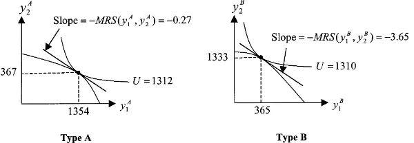
Fig. 1. Unboundedly rational choices for subject types A and B.
in the process of optimizing should choose to produce more Good 1 and less Good 2-a result which is intuitively sensible given that decision costs must be paid in terms of Good 1.
To make trade potentially attractive, two types of subjects were introduced. ‘Type A’ sub-jects were given the production parameters (a,b) = (550,0.0001), while ‘Type B’ subsub-jects were given (a,b) = (2000,0.005). Given the log linear utility function used, for an unbound-edly rational self-sufficient Type A subject, the marginal rate of substitution of the optimal production/consumption bundle would beMRS(y1A, y2A) = (y2A/y1A) = (367/1354) = 0.27, while the same for the Type B subject would be MRS(y1B, y2B) = (y2B/y1B) = (1333/365) = 3.65. BecauseMRS(y1A, y2A) < MRS(y1B, y2B), there were potentially a wide range of mutually beneficial barter offers involving the transfer of Good 1 from the Type A subject to the Type B subject in exchange for Good 2. On the other hand, two subjects of the same type would not easily find a mutually beneficial barter trade. Fig. 1 presents the two Robinson Crusoe equilibrium production/consumption bundles for the two types, assuming unbounded rationality.
3. Barter
Subjects entered the experimental economy sequentially. The first subject had to be self-sufficient. Subsequent subjects could barter with those who had previously participated, with the computer bargaining on behalf of the previous participants. Specifically, given the post-production profile(y1n, y2n), subject n could initiate a barter transaction by first selecting a potential trading partner from the population of subjects who had already entered the economy, say subject k. Next, subject n could make an offer (e1,e2) to subject k, where ehis
the excess demand for good h by subject n. Let Ui,j denote the utility achieved by subject
i achieved during period j. If the computer accepts subject n’s offer on behalf of subject k after subject n has used D seconds to produce and trade, then subject n would achieve
the utility levelUn,n = U1(y1n−D+e1)+U2(y2n +e2)and subject k would achieve
the utility levelUk,n =U1(y1k−e1)+U2(y2k−e2). No decision cost is figured into the
utility calculation of subject k, a simplifying assumption that implies subject n finds subject
k without any effort on the part of subject k. Subject k had achieved the utility level Uk,n−1
behalf of subject k if and only if Uk,n> Uk,n−1. Of course, subject n should only consider
offers whereUn,n> U1(y1n−D)+U2(y2n).
4. Trade through a store
Successful barter requires that a subject both solve the ‘double coincidence of wants’ problem and negotiate mutually beneficial terms of trade. Both of these tasks can be time consuming. Consequently, one explanation for the development of trading intermediaries is that they reduce the decision costs associated with barter.
Consider an intermediary that, for convenience, is called a ‘store.’ A store is defined by a Good 1 wholesale price q1, a Good 2 wholesale price q2, and a markup m. A store buys
at wholesale prices and sells at retail prices. The retail prices of Good 1 and Good 2 are marked up wholesale prices, calculated as p1≡[1 + m]q1and p2≡[1 + m]q2. If the subject
buys Good 2 from the store,ρ1≡(q1/p2) = (q1/[1 + m]q2) gives the number of units of Good
2 that the subject will receive from the store for each unit of Good 1 delivered to the store. If the subject buys Good 1 from the store,ρ2≡(p1/q2) = ([1 + m]q1/q2) gives the number
of units of Good 2 that the subject must deliver to the store for each unit of Good 1 received from the store.
Whether and how the subject should use the store depends upon the relationship between the trading rates offered by the store and the marginal rate of substitution of the subject’s post-production profile. Three mutually exclusive cases emerge:
• Case 1: If MRS(y1,y2)< ρ1, trade Good 1 for Good 2 through the store;
• Case 2: If MRS(y1,y2) >ρ2, trade Good 2 for Good 1 through the store;
• Case 3: Ifρ1≤MRS(y1,y2)< ρ2, do not trade through the store.
If either Case 1 or Case 2 applies, trading through the store can improve the subject’s welfare. Assuming D represents the decision costs which must be expended for the subject to produce and find an optimal trade through the store, the subject’s problem is to choose
c1and c2so as to:
MAXU =U1(c1)+U2(c2)
subject to
c2= y2+ρ1[y1−D−c1] if Case 1 applies; or
c2= y2+ρ2[y1−D−c1] if Case 2 applies.
Given the log linear utility function, the solutions are c1= ((y2/ρ1) + y1−D/2), c2= (y2+
ρ1[y1−D]/2) if Case 1 applies and c1= ((y2/ρ2) + y1−D/2), c2= (y2+ρ2[y1−D]/2), c2=
y2+ρ2[y1−D]/2 if Case 2 applies.
As the markup m increases,ρ1decreases andρ2increases, reducing the volume of trade
A special case is the case where m = 0. With a zero markup, wholesale and retail prices would be equal andρ1=ρ2. Case 3 would hold only if by chance MRS(y1,y2) =ρ1=ρ2,
meaning all subjects would almost surely find trading through the store more attractive than self-sufficiency. To be viable with this zero markup, the store would have to be able to operate without incurring any costs and would be restricted to earning zero profits. This special case is that implicitly assumed in standard general equilibrium model where trade is mediated exclusively by a price system.
Here, a more general case is considered by assuming that the store-owner must pay costs equal to C1≥0 units of Good 1 and C2≥0 units of Good 2 to operate the store. After paying
these costs and meeting all of the trading desires of its customers, the store owner is allowed to keep any remaining inventory as profits. As the costs C1and C2increase from zero, the
markup must also increase in order for the store to be viable. The increase in the markup would make Case 3 (no trade through the store) more likely and would reduce the volume of trade through the store under cases 1 and 2. That is, increases in the costs of providing intermediation reduce the extent to which self-sufficient subjects can benefit from mediated trade.
An increase in the wholesale price ratio q1/q2increases bothρ1andρ2. This causes all
subjects trading with the store to reduce their consumption of Good 1 and increase their consumption of Good 2. Subjects under Case 1 sell more Good 1 to the store, while subjects under Case 2 buy less Good 1 from the store. Conversely, subjects under Case 1 buy more Good 2 from the store, while subjects under Case 2 sell less Good 2 to the store.
An increase in the decision cost level D decreases the optimal consumption levels of both goods, implying a reduction in mediated trade.
5. Opening a store
In the experiment, no store exists at the outset. If intermediation is to occur, it must arise endogenously. As an alternative to barter or trading through an existing store (if one were in existence), subjects could attempt to open a store.
The store attracts inventories of the two goods by paying the wholesale prices q1and
q2. Out of this inventory, the store must first deliver to subjects their desired purchases of
Goods 1 and 2. With a positive markup, it is conceivable that the store could generate excess supplies of each good. Let the functions E1(m,q1/q2) and E2(m,q1/q2) denote the excess
supplies as they depend upon the markup m and the wholesale price ratio q1/q2. Out of
these excess supplies, the store must pay its operating costs C1and C2. Thus, after it pays
its costs and meets all of the subjects’ trading desires, the store’s remaining inventories of the two goods can be represented by I1= E1(m,q1/q2)−C1and I2= E2(m,q1/q2)−C2.
To obtain explicit representations for E1(m,q1/q2) and E1(m,q1/q2), consider some
addi-tional simplifying assumptions. Suppose (1) trading through the store is the only alternative to self-sufficiency; (2) all subjects optimize with D = 0, and (3) the number of type A sub-jects, nA, is equal to the number of Type B subjects, nB, so that n = 2nA= 2nBgives the
number of subjects in the economy. It then follows that the store’s inventories I1and I2are
I1
Note that I1 and I2are not monotonic functions of the markup m. When the markup
increases, Type A subjects sell less Good 1 to the store, while Type B subjects sell less Good 2. These responses reduce the store’s inventories of each good. However, the store’s inventories of each good are enhanced by the fact that Type A subjects buy less Good 2 from the store, while Type B subjects buy less Good 1. The partial derivative∂I1/∂m indicates
that an increase in the markup generates an increase in I1whenm <
q
(y1A/y1B)−1, with
I1decreasing for larger markups. Similarly, the partial derivative∂I2/∂m indicates that an
increase in the markup generates an increase in I2 when m <
q
(y2B/y2A)−1, with I2
decreasing for larger markups.
The store’s most pressing problem is viability, which requires I1≥0 and I2≥0. Note that
if m = 0 and (q1/q2) = 1, then E1= 0 and E2= 0 so that I1=−C1and I2=−C2. In this case,
the store is viable only if C1= 0 and C2= 0. This outcome is the standard general equilibrium
solution. However, if there are costs to operating the store, then the store cannot be viable with a zero markup. When C1> 0 or C2> 0, the store must generate an excess supply of
one of the good without generating an excess demand for the other good. Note that E1
is an increasing function of q1/q2,while E2is decreasing. Thus, as q1/q2increases from
(q1/q2) = 1 with m = 0, E2becomes negative. Conversely, as q1/q2decreases from (q1/q2) = 1
with m = 0, E1becomes negative. Therefore, as long as m = 0, there is no adjustment the
store can make in the wholesale price ratio so that it can cover either C1> 0 or C2> 0.
For a given wholesale price ratio q1/q2, E1 and E2increase as m increases from zero.
Thus, there must exist a range of markup levels where the store can at least pay portions of any positive operating costs C1and C2. However, because E1and E2are decreasing in m
once the critical markup levels (given above) are reached, there is no guarantee that a viable markup level exists for a given population n of subjects.
Yet, as long as q1/q2and m are set so that E1and E2are positive, the store must eventually
become viable as the population of subjects increases. Mathematically, this follows from the fact that I1and I2are each increasing in n as long as E1and E2are each positive. The
intuition is that, if the number of transactions is large enough, any level of operating costs can be covered by the store if the store is netting a positive return on each transaction.
Since the store-owner can consume the remaining inventories I1and I2, store ownership is
potentially lucrative. Given his or her own post-production bundle (y1,y2), a subject seeking
to open a store could move beyond the viability goal and choose m and q1/q2 so as to
maximize U = U1(y1−D + I1) + U2(y2+ I2), where D is the decision cost required to first
Recognizing the potential for competition, another approach to determining the markup and wholesale price ratio would be to assume that the store-owner would act so that no other store-owner could viably enter the market. This ‘contestable markets’ solution would imply that m and q1/q2are set for a given population of n subjects so that E1= C1and E2= C2.
(Note that this contestable markets solution is the same as the standard general equilibrium solution if D = C1= C2= 0.)
6. Experimental procedure
For an individual subject, participation in the experiment consisted of playing the ‘Pro-duction and Trade Game,’ the computer game comprised of the four trading options de-scribed above. Prior to participating, a subject read a set of instructions and played four standard practice games, one practice game for each trading option.4 The practice games were necessary in order for subjects to become familiar with the options and the associated keystrokes. Questions asked by subjects about ‘procedure’-how to do something-were an-swered, but any questions about ‘performance’-what should be done or what is good-were not answered. In answering any question, every effort was made to not bias the subject toward any one of the four trading options.
Each subject played 10 independent games, with the choices and environmental param-eters being recorded. Thinking of each game as participation in a different experimental economy, the experiment resulted in the formation of 10 experimental economies. The first economy consists of relatively inexperienced participants, while the 10th economy consists of relatively experienced subjects.
When playing the Production and Trade Game, a subject first had to produce. The subject was shown the maximum amount of Good 2 that could be produced and was asked to choose a Good 2 production level. Upon receiving the Good 2 choice, the computer calculated the production of Good 1, assuming efficient production. (That is, the production combination was on the production possibilities frontier described in Section 2.) The Good 1-Good 2 production bundle was then shown to the subject, along with its associated utility level. The subject then had to either accept or reject this ‘provisional’ production choice.
By rejecting provisional production choices, the subject could compare the utility of various production alternatives. However, such comparison was costly because Good 1 was taken from the subject in proportion to amount of decision time used. As a subject paused to contemplate, the provisional inventory of Good 1 and the provisional utility level each decreased on the computer screen, allowing the subject to observe the negative impact of the decision cost.
After producing, a subject could trade. The computer asked the subject to choose a trading option from four alternatives: (1) a no-trade ‘consumption’ option, (2) a ‘barter’ option, (3) a ‘trade through a store’ option, and (4) an ‘open a store’ option. While considering or pursuing any of these options, the subject had to pay the decision cost.
The consumption option allowed a subject to be self-sufficient. Upon choosing this option, the computer simply showed the subject the utility level achieved and then started a new
game. The first subject could only choose this option because there were no other potential trading partners. All other subjects could choose the consumption option and the other three options.
When the barter option was selected, the subject was first shown how many previous subjects had played the game and asked to select a trading partner. (No information was given about these potential trading partners.) After selecting a trading partner, the subject was shown his or her own inventories of Good 1 and Good 2 and was asked to choose whether the desire was to trade away Good 1 and receive Good 2 in return, or vice versa. Next, the subject had to make an offer consisting of how much to trade away of the one good and how much desired in return of the other good. The computer then told the subject whether or not the trading partner accepted the offer. As explained in detail in Section 3, the offer was rejected if the computer found that the trading partner would be made worse off by the trade. In this case, the trading part of the game restarted, meaning the subject had to again choose from among the trading options. If the barter offer was accepted by the partner, the computer showed the subject his or her own utility level ‘with the trade’ and ‘without the trade,’ asking the subject to accept or reject the trade. If the subject accepted the barter trade, the computer showed the resulting utility level and then moved on to a new game. If the trade was rejected, the trading part of the game restarted.
When the ‘trade through the store’ option was selected, the computer first checked to see if a store was in existence. If no previous subject had opened a store, then the computer printed the words ‘no store exists’ and restarted the trading part of the game. If a store did exist, the computer first showed the subject his or her inventories of Goods 1 and 2 and asked the subject to choose whether to trade away Good 1 and receive Good 2 in return, or vice versa. Then, the computer displayed the store’s inventories of Goods 1 and 2, along with the store’s terms of trade. If a subject tried to buy more of either good than the store had in its inventories, the computer so informed the subject and restarted the trading part of the game. If the store had the inventory to mediate the subject’s desired trade, then the subject was shown his or her own utility levels with and without the trade, asking the subject the to accept or reject the trade. Upon acceptance, the computer displayed the utility level achieved and started a new game. Upon rejection, the trading part of the game was restarted.
partner found the store’s terms of trade as attractive as those being received through barter, and who were better off being self-sufficient due to an excessive store markup.
To determine whether a prior subject could benefit by trade through the store, the computer calculated what the subject’s optimal trading levels would be, given the store’s prices. Then, the computer compared the utility level associated with optimally trading through the store with the subject’s existing utility level. If the former utility level was higher, then the subject was assumed to trade through the store in the optimal way. This optimality assumption is obviously inconsistent with the fact that subjects who chose to trade through the store when actually playing the game tended to make suboptimal trades. However, this assumption allows for sequential play and also provides experimental control in that the changes in choices of prior subjects made by the computer are based totally upon the market implications of the choice of the current subject, as opposed to changes in cognition. For future work, it would be interesting to design an experiment with a growing population of subjects where the participants could interact and make their own adjustments as the economy evolved. Although data collection and control of the conditions would be more troublesome, such an approach would allow one to observe the ‘gamesmanship’ associated with trade development.
To open a store successfully, a subject had to find wholesale prices and a markup level that enabled the execution of all trades desired by its customers and the payment of operating costs. After subtracting the operating costs, the computer calculated and displayed the inventories attracted by the ‘provisional’ store. If the wholesale price and markup choices were not viable, it was because they either did not attract enough Good 1, or Good 2, or both. In this case, the subject would see that the inventory of at least one of the goods was negative, and the computer would re-start the trading part of the game. If the provisional store was viable, the subject was shown the utility level associated with store ownership as compared to self-sufficiency, giving the subject the opportunity to accept or reject the trade. Upon acceptance, the computer showed the resulting utility level and then started a new game. Upon rejection, the trading part of the game restarted.
7. A digression on experimental incentives
Each subject’s goal was to maximize utility. No monetary incentives were used to motivate subjects to make choices according to the preferences programmed into the computer. The excitement of the game, or ‘game value’ as Smith (1982) calls it, was relied upon to appropriately induce subjects to perform. Because monetary payments have become common in experimental work, the reasons for not providing payments here are explained in some detail.
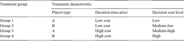
Table 1
Experimental treatments
Treatment group Treatment characteristic
Player type Decision-time price Decision cost level
Group 1 A Low cost Low
Group 2 B Low cost Medium-low
Group 3 A High cost Medium-high
Group 4 B High cost High
task without being paid. The test indicated that the pay neither led to significantly better performance nor a reduction in the variance of performance.
Second, a monetary payment can have unintended effects that bias a subject’s behav-ior inappropriately. Hogarth and Reder (1986, p. 196) cite a number of studies in which, ‘contrary to economic theory, greater incentives have been shown to lead to less rather than more ‘rational’ behavior.’ If the experiment’s game value suggests a monetary incentive is not necessary, the prudence of providing one is questionable.
Third, the decision-making task in this experiment is quite complex. As noted by Davis and Holt (1993), ‘Inconsistent or variable behavior is not necessarily a signal of insufficient monetary incentives. No amount of money can motivate subjects to perform a calculation beyond their intellectual capacities.’ Because variations in behavior will be observed when-ever a task is as complex as the one examined here, the ‘saliency’ of any monetary payment system could be questioned.
Fourth, the treatments within the experiment, described in the next section, each involve the same control or lack of it. Roth (1995, p. 79) notes that ‘a choice an individual makes is sometimes sensitive to the way it is presented.’ Consequently, ‘the most reliable comparisons are ‘within experiment’ comparisons, in which the effect of a single variable can be assessed within an otherwise constant environment.’ While the general behavior of subjects is of some interest, the focus here is on the within experiment comparison of treatment groups that allow us to examine the impact of a change in the decision cost level.
8. Treatments
The decision-time price for the high cost cell was set high enough so that its affect outweighed the type effect. That is, a Type A subject in treatment Group 3, while more adept at producing the good needed to pay the decision cost, would find the use of decision-time more costly in terms of foregone utility that a Type B subject in Group 2. Consequently, the four treatment groups were ranked by decision cost level as shown in Table 1.
The participating subjects were all undergraduate students at the University of Nevada. Sequential participation meant that the population of the experimental economy increased by one each time a new subject played. Twenty-five subjects participated in the low cost cell and 25 subjects participated in the high cost cell. Treatment groups 1 and 3 each contained 13 subjects, and treatment groups 2 and 4 each contained 12 subjects.
9. Results
The data obtained were recorded in three data sets-the ‘Subject Data Set,’ the ‘Economy Data Set,’ and the ‘Store Data Set.’
9.1. Subject behavior
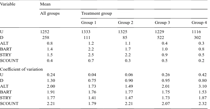
The Subject Data Set contained the trading choices made by subjects. The variable S identified the subject number, running from 1 to 25; R denoted the round of play (or game number), running from 1 to 10; D denoted the decision cost incurred by the subject, measured in units of Good 1; and U denoted the subject’s utility level. ALT was the number of alternatives considered prior to accepting a production alternative. BART was the number of barter attempts. STRY was the number of attempts to open a store. SCOUNT was the number of attempts to trade through a store. Table 2 presents some descriptive statistics on these variables.
How did a change in the decision cost level affect performance? The mean utility level
U decreased and the coefficient of variation for U increased across the four treatment
groups. At a 5 percent level of significance, the differences between groups 1 and 2 were not statistically significant, but the means and coefficients of variation for groups 3 and 4 were significantly different from each other and significantly different from groups 1 and 2. To summarize, an increase in the decision cost level led to poorer and more variable
performance.
Table 2
Subject behavior and performance
Variable Mean
All groups Treatment group
Group 1 Group 2 Group 3 Group 4
U 1252 1333 1325 1229 1116
D 258 111 85 522 302
ALT 0.8 1.2 1.1 0.4 0.3
BART 1.4 2.2 1.7 1.0 0.8
STRY 1.5 2.5 2.2 0.9 0.5
SCOUNT 0.4 0.7 0.3 0.5 0.2
Coefficient of variation
U 0.24 0.04 0.06 0.26 0.42
D 1.30 0.75 0.90 0.95 0.80
ALT 2.00 1.73 1.49 2.01 3.10
BART 1.91 1.76 1.77 1.75 1.53
STRY 1.77 1.41 1.47 1.73 1.87
SCOUNT 2.21 1.79 2.21 2.07 2.32
failed to use their decision time effectively, while subjects facing lower decision costs tended to use decision time effectively.
The fact that the average subject in Group 3 or 4 tended to achieve a utility level below what could have been achieved through self-sufficiency does not necessarily indicate irrational behavior. A priori, no subject could know whether or not they would be effective at using decision time to obtain gains from trade. A subject who is ineffective must unfortunately learn of the ineffectiveness by experiencing losses in utility rather than gains. All subjects should economize on decision time because it is valuable. However, if the subjects are learning to use decision time according to how it bears fruit, then subjects who use decision time less fruitfully should be observed economizing on decision time more intensely. The price of decision time for subjects in groups 3 and 4 was 10 times higher than for groups 1 and 2. Thus, we must divide the mean decision costs shown for groups 3 and 4 in Table 2 by 10 in order to get the decision time used. The mean decision times for groups 1–4 were 111, 85, 52, and 30, respectively. That is, subjects who tended to use decision time
less effectively economized on it more intensely.
What did subjects do with the decision time they used? The means for the variables ALT, BART, STRY, and SCOUNT give some indication. Attempts to open a store were most
frequent, followed closely by attempts to barter. The comparison of production alternatives
and attempts to trade through the store were significantly less common. This pattern was the same for all the groups. The mean for each of the four variables tends to decline across the groups 1 through 4, an indication that subjects in higher cost groups were economizing on decision time by comparing fewer production alternatives and making fewer attempts to trade. The increased variability of STRY for groups 3 and 4 indicates that the high decision cost environment discouraged the store opening efforts of some more than others.
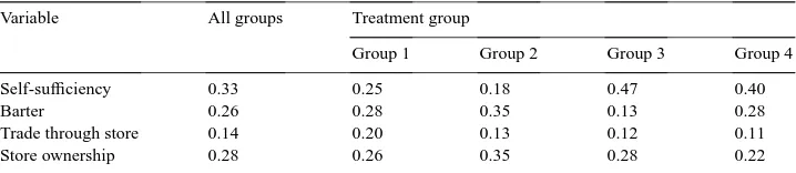
Table 3
Post-production trading decisions (proportion of subjects, by group) Variable All groups Treatment group
Group 1 Group 2 Group 3 Group 4
Self-sufficiency 0.33 0.25 0.18 0.47 0.40
Barter 0.26 0.28 0.35 0.13 0.28
Trade through store 0.14 0.20 0.13 0.12 0.11
Store ownership 0.28 0.26 0.35 0.28 0.22
post-production choices ultimately made using self-sufficiency, barter, trade through a store owned by another subject, and trade through a self-owned store. Self-sufficiency was most
common in the high cost groups and overall. Barter and store ownership was more common in the low cost groups.
Trading through an existing store was least common in every group. This result is sur-prising in that trading through an existing store was easy for subjects compared to opening a store or bartering. The primary explanation for the lack of trading through an existing store was that the inventories available at the store depended upon the behavior of the subject who had opened the store, and these inventories were typically small. Given a small inventory, a subject trying to trade through the store often could not buy enough of the desired good to obtain a significant increase in utility. Because the stores typically had small inventories, the potential utility gain was usually larger via barter or opening a store than trading through a store.5 It was not difficult for most subjects to discover this fact.
Table 4 contains the results of 10 regressions aimed at explaining the observed variation in the utility earned by the 50 different subjects in the 10 rounds of play. The explanatory variables examined include dummy variables G1–G4, respectively representing decision cost treatment groups 1–4, the number of rounds of experience R, the decision cost incurred
D, the number of subjects S, and interactions between these variables. The regressions
indicate the following:
Greater experience did not generally lead to improved performance (Regressions 2 and 6). A larger population of subjects resulted in improved performance, especially when decision
time was more valuable (Regressions 3, 5, and 9).
Incurring additional decision cost generally led to worse performance, especially when decision time was more valuable. (Regressions 4, 5 and 8).
Incurring additional decision cost was more fruitful when the population of subjects was relatively large than when the population of subjects was relatively small, especially when decision time was more valuable (Regressions 7 and 10).
With regard to the last finding, an increase in the number of subjects enlarges the potential market, making it easier and more profitable to open a store. This makes it more likely that incurring additional decision cost will be fruitful. Regressions 7 and 10 indeed indicate that subjects who entered the experimental economy later, when the economy had a larger
population, were able to obtain utility gains by incurring decision cost, especially subjects in the high decision cost treatment groups 3 and 4.
To examine how a subject’s utility depended upon which trading option the subject ultimately chose, consider the equation,
U=1361G1
(38.2)∗∗∗ +1308G2(36.7)∗∗∗ +1213G3(42.6)∗∗∗ +1081G4(36.9)∗∗∗ +39.8TR1(1.13) +103TR2(2.12)∗∗∗
+202TR3
(6.16)∗∗∗ −4.97ALT(0.59) −17.9BART(3.41)∗∗∗ −14.7STRY(2.86)∗∗∗ −48.3SCOUNT(2.84)∗∗∗
estimated using least squares. The standard errors are shown in parentheses. A standard error with three stars indicates significance at the 1 percent level, while no stars indicates insignificance at the 10 percent level. Respectively, TR1, TR2, and TR3 are dummy vari-ables for consumption choices ultimately made using barter, trade through a store owned by another subject, and trade through a self-owned store. (A fourth dummy variable TR0 was defined for self-sufficiency and is used below.) The positive coefficients on TR2 and TR3 indicate that subjects who ultimately chose to trade through an existing store or open their own store, were significantly better off that subjects who were self-sufficient. To the contrary, the statistically insignificant coefficient on TR1 indicates that subjects who ulti-mately engaged in a barter transaction were not significantly better off than the self-sufficient subjects. Overall, the regression indicates that, controlling for differences in decision cost
levels and differences in search efforts, it was beneficial for a subject to move away from self-sufficiency and barter toward mediated trade.
9.2. Evolution of the experimental economy
The Economy Data Set is an evolving data set that keeps track of how the trading choices of subjects affect the economy as new subjects are added to the population. It contains two sub-economies: a ‘low decision cost economy’ identified by the dummy variable LC, and a ‘high decision cost economy’ identified by the dummy variable HC. The low decision cost economy included the 25 subjects in groups 1 and 2, while the high decision cost economy included the 25 subjects in groups 3 and 4.
A given economy, say the low decision cost economy, evolved in 25 steps, with one step in the evolution occurring each time a new subject participated in the experiment. Indexing these evolutionary steps by S, let Economy-S denote the economy after subject S has participated. Using this notation, Economy-1 is a data set that provides information on the self-sufficient behavior of the first subject. Because trade can occur between subject 1 and subject 2, the variables associated with subject 1 in Economy-2 may take on different values than in Economy-1. Most significantly, the variable U will increase if Subject 2 makes a trading decision that benefits subject 1. As Economy-1 evolves into Economy-25, the patterns of trade development and resulting changes in welfare are captured.
subject,Dremained equal to the decision cost D. Once the computer traded on behalf of the resident subject,Dwas set equal to zero and remained equal to zero. Intuitively, the computer acted as an agent for resident subjects, an agent who can trade without incurring decision costs.
To examine how trading choices were affected by various factors, consider the following four equations, obtained from logit estimation.
For each regression, there were 6500 observations [2 sub-economies×10 rounds per sub-ject×(1 + 2 +. . .+ 25) subjects in the economy during the economy’s 25 states of evolu-tion]. The respective number of correct cases predicted by the models for TR0, TR1, TR2, and TR3 were 5865, 5768, 5379, and 6185. By including interactions between the variables of interest-R, S, and STAY-and the group dummies LC and HC, the regressions allow dif-ferences between the high decision cost economy and low cost economy to be recognized. Only those explanatory variables and interactions that were significant at a 5 percent level are presented here.6 The regressions indicate
Subjects moved away from barter and self-sufficiency toward trading through a store as the economy evolved.
Subjects in the low decision cost economy moved away from self-sufficiency at a faster rate than subjects in the high decision cost economy.
Subjects in the low decision cost economy were more likely to barter, but also moved away from barter more readily as experience was gained and as additional subjects entered the economy. Store ownership was less likely as the term of stay in the economy lengthened Fig. 2 gives a visual perspective of the movement of traders toward mediated trade as the economy evolved due to the increase in the population of subjects.
As noted in Table 1, the mean utility level for subjects groups 1, 2, 3, and 4 were 1333, 1324, 1229, and 1116. These means were calculated using the data for the period when each subject entered the economy. Consequently, they do not recognize the benefits obtained by resident subjects as participating subjects opened new stores. The mean utility levels for all subjects in Economy-25 reflect the benefits of the development of stores. The means for the four groups in Economy-25 were 1345, 1338, 1325, 1335. Notice that the development
of mediated trade not only increased the utility levels, but the utility levels also tended to
converge. These results should not be surprising in that they are largely the result of the
assumption that resident subjects trade through new stores optimally with zero decision cost whenever such trade is Pareto improving. Nonetheless, they illustrate how the development of mediated trade can be beneficial, particularly in a high decision cost environment.
9.3. Store behavior
Like the Economy Data Set, the Store Data Set is evolving data set. The Store Data Set provides information about the development of the store (i.e. mediated trade). The variables
q1and q2are the store’s wholesale prices for Good 1 and Good 2. M is the store’s markup
percentage. EXIST is a dummy variable which takes on the value 1 when a store exists and 0 otherwise. Analogous to the notation used for the Economy Data Set, let Store-S denote the state of the store after subject S has participated. Again, LC and HC are dummy variables used to distinguish the low decision cost economy from the high decision cost economy.
In the low decision cost economy, the first store was opened by subject 9. Stores were not open in each of the 10 rounds of games until subject 14 had played. The average subject opened 3.0 stores (in the 10 rounds). Alternatively, in the high decision cost economy, the first store was opened by subject 5; stores were not open in each of the 10 rounds of games until subject 18 had played; and the average subject opened 2.6 stores. Note that subjects
in the low decision cost economy more quickly exhausted the opportunities to open the first store and opened more stores on average. The fact that a store emerged earlier in the high
decision cost economy illustrates the role luck can play in trial and error search.
To consider how the probability of opening a store is affected by various factors, consider the equation: obtained using a logit estimation. The model predicts 461 correct cases for 500 observations. The regression indicates the following:
The probability of opening a store increased as the number of subjects increased and as the number of rounds of experience increased.
Additional subjects (i.e. additional opportunity) and additional experience increased the likelihood of opening a store more substantially in the low decision cost economy than in the high decision cost economy.
To consider how the store’s markup evolved as additional subjects entered the economy and as subjects gained experience, the following equation was estimated by least squares using only the 334 (out of 500) observations where a store existed:
M=0.35LC
The coefficients on LC and HC are the predicted markups for the initial stores opened in the two economies-35 percent for the first store in the low decision cost economy and 110 percent for the first store in the high decision cost economy. The coefficients on S∗LC
and S∗HC indicate that the markup decreased as additional subjects were added to the
affect the markup in the low cost economy. However, in the high decision cost economy, subjects reduced the markup by 2 percentage points per round.
Fig. 3 gives a visual perspective of how the markup levels evolved in the low decision cost economy relative to the high decision cost economy. For each economy, 250 markup levels are plotted. As noted earlier, each of the 10 rounds of play for a subject can be thought of as participation in 10 different economies. The first 10 markups shown are the store markups for these 10 economies after the participation of subject 1. This presentation continues so markups 241–250 are the store markup levels for the 10 economies after the participation of subject 25. A markup level does not exist when a store does not exist. To allow identification in Fig. 3, an arbitrarily high markup (120 percent) was assigned to the instances where no store existed. (Intuitively, one can think the nonexistence of a store as a situation where the markup is so high that mediated trade is prohibitively expensive.) Equipped with this understanding of how the data is presented in Fig. 3, one can observe how subjects took advantage of the opportunities to bring stores into existence and how subjects competed with existing stores to drive down markups.
To examine the evolution of the store’s wholesale price ratio, consider the following equation, which has estimated by least squares using only the 334 observations where a store existed:
q1
q2 =
0.80LC
(0.013) +0.02S ∗LC
(0.002) +0.81HC(0.016) +0.003S ∗HC (0.001)
The coefficients on LC and HC are the predicted price ratios for the first store opened in each economy-0.80 for the low decision cost economy and 0.81 for the high decision cost economy. While these estimates are statistically equivalent, the coefficients on S∗LC
and S∗HC indicate that the price ratio tended to increase more quickly in the low decision
cost economy than in the high decision cost economy. As mentioned in Section 2, the standard general equilibrium solution for this economy is associated with a zero markup and a wholesale price ratio equal to one. The regression indicates that the each experimental economy evolved toward the standard general equilibrium solution, with the low decision cost economy doing so more quickly.
10. Discussion
these three conditions, while necessary, are not sufficient. This pilot study illustrates that another necessary condition for mediated trade is that the market be large enough so that, in addition to the store’s operating costs, the decision costs of those opening the mediating institution can be financed. Like operating costs, decision costs act as a barrier to mediated trade.
The experiment also highlights a characteristic of prices that is not readily apparent in the typical economic model. Prices are not merely accounting conventions. They are the tools used by intermediaries, together with markups, to make a market. When the size of the market is large relative to the competition in the intermediation sector, the set of viable prices is large, as is the set of viable markups. As competition decreases markups, the set of viable prices decreases. Together, competition and a growing market can move a real world economy toward the equilibrium defined by general equilibrium theory. A growing market drives the cost of trade toward zero by allowing operating and decision costs to be financed with a lower markup. Competition drives retail prices toward wholesale prices by driving markups toward zero.
The experiment illustrates that, although the development of trade is good on average, it is not universally beneficial. To take advantage of new trading opportunities, some subjects found it beneficial to abandon existing trade arrangements. Those left behind were not always able to find new trading opportunities as attractive as the old arrangements. In particular, as trade mediation develops and markups are reduced, relatively weak bargainers in barter arrangements tend to be helped, while relatively strong bargainers tend to be hurt. (See Bose and Pingle (1995) for a theoretical discussion of how mediated trade can provide insurance against poor bargaining.) In addition, when an intermediary is displaced by a new intermediary with a lower markup, those trading through the intermediary are helped but the owner of the displaced intermediary is hurt.
Finally, it is notable that subjects in the experiment often engaged in search to the point of it being detrimental. The use of decision time was not productive at the margin for the average subject, regardless of how the time was used. However, the welfare of the average subject improved as the economy evolved. If subjects had significantly reduced their search efforts by limiting their decision costs, the learning responsible for the societal improvement might not have taken place. This presents a paradox for society: While incurring decision costs may often be wasteful, obtaining societal improvement may require that decision costs be incurred. Of course, more successful societies will more adeptly motivate decision-makers to make decision costs fruitful and possess institutions that can adapt so as to incorporate the fruits of decision costs. Nonetheless, fruitlessly incurring decision costs may be a required ingredient in any recipe for societal improvement.
References
Baumol, W., Quandt, R., 1964. Rules of thumb and optimally imperfect decisions. American Economic Review 54, 23–46.
Bose, G., Pingle, M., 1995. Stores. Economic Theory 6, 251–262.
Conlisk, J., 1980. Costly optimizers and cheap imitators. Journal of Economic Behavior and Organization 1, 275–293.
Conlisk, J., 1996. Why bounded rationality? Journal of Economic Perspectives 34 (2), 669–700.
Day, R., 1984. Disequilibrium economic dynamics. Journal of Economic Behavior and Organization 5, 57–76. Day, R., Pingle, M., 1991. Economizing economizing. In: Franz, R., Singh, H., Gerber, J. (Eds.), Handbook of
Behavioral Economics. JAI Press, Greenwich, CT, pp. 511–524.
Day, R., Pingle, M., 1996. Modes of economizing behavior: experimental evidence. Journal of Economic Behavior and Organization 29, 196–209.
Davis, D., Holt, C., 1993. Experimental Economics. Princeton University Press, Princeton, NJ. Debreu, G., 1959. Theory of Value: An Axiomatic Analysis of Economic Equilibrium. Wiley, New York. Hogarth, R., Reder, M., 1986. Editors’ comments perspectives from economics and psychology. Journal of Business
59, S185–S208.
Pingle, M., 1992. Costly optimization: an experiment. Journal of Economic Behavior and Organization 17, 3–30. Pingle, M., 1995. Imitation versus rationality: an experimental perspective on decision making. Journal of
Socio-Economics 24 (2), 281–315.
Pingle, M., 1997. Submitting to authority: an experimental analysis of its effect on decision-making. Journal of Economic Psychology 18, 45–68.
Roth, A., 1995. Introduction to experimental economics. In: Kagel, J., Roth, A. (Eds.), The Handbook of Experimental Economics. Princeton University Press, Princeton, NJ, pp. 3–109.
Simon, H., 1955. A behavioral model of rational choice. Quarterly Journal of Economics 69, 99–118.
Simon, H., 1978. Rationality as a process and product of thought. American Economic Review, Papers and Proceedings 68, 1–16.
Smith, V., 1982. Microeconomic systems as an experimental science. American Economic Review 72, 923–955. Varian, H., 1978. Microeconomic Analysis. W.W. Norton & Co., New York.