International Review of Economics and Finance 8 (1999) 467–478
Short-run and long-run demand for financial assets
A microeconomic perspective
Jan Tin*
Housing and Household Economic Statistics Division, U.S. Bureau of the Census, 6066 Oust Lane, Woodbridge, VA 22193, USA
Received 21 July 1998; accepted 11 January 1999
Abstract
One of the major issues associated with the short-run aggregate money demand is that the speed of adjustment has become very slow or even negative when the post-1973 periods are included in regressions. This implies that the long-run effects of income, wealth, or the opportu-nity costs on money demand may be so large that a small change in any of these variables would lead to unreasonably large fluctuations in asset demand. Using microeconomic data from the Survey of Income and Program Participation conducted by the U.S. Bureau of the Census, this study finds that the speeds at which individuals adjust their actual quantities of financial assets toward the desired levels are actually quite fast. In the long run, there is no indication that the desired quantities of monetary assets fluctuate widely whenever an explana-tory variable is disturbed. 1999 Elsevier Science Inc. All rights reserved.
JEL classification:E41
Keywords:Asset demand; Speed of adjustment; SIPP
1. Introduction
In the literature, the relationship between the short-run and long-run money demand is often linked by the speed at which individuals adjust their short-run actual quantities of financial assets toward the long-run desired levels. In the long run, the effects of income, wealth, and opportunity costs on asset demand are inversely related to the speed of adjustment; a slower speed of adjustment implies larger coefficient estimates of asset demand. Theoretically, the impact of each explanatory variable on long-run
* Corresponding author. Tel.: 301-457-8302. E-mail address: [email protected] (J. Tin)
asset demand could become infinite as the speed of adjustment approaches 0, while a negative speed of adjustment would render the long-run asset demand inconsistent with economic theories. In reality, however, it is questionable that these two conditions have ever existed in any economy.
Empirically, aggregate money demand studies up to the early 1970s (e.g., Chow, 1966; Goldfeld, 1973) generally found the speed of adjustment to be reasonable. However, subsequent researchers such as Garcia and Pak (1979), Friedman (1978), Wenninger and Sivesind (1979), Hafer and Hein (1980), Milbourne (1983), Barnett et al. (1984), Hafer and Thornton (1986), Goldfeld and Sichel (1987), and others have found the speed of adjustment to be quite slow or even negative when post-1973 monetary aggregates are employed in short-run money demand studies. Whether this is also the case at the individual level is not quite clear, however, and an empirical examination of the microfoundations of the short-run and long-run money demand is worthwhile and may provide valuable insights into the issues related to aggregate money demand.
In this article, we attempt to show that the short- and long-run demands for financial assets by individuals are consistent with consumer theories. Findings in this study indicate that when microeconomic data on asset demand, rates of return, wealth, and demographic variables are applied directly to economic theories without the complications of the identification problem (Laidler, 1977; Cooley & LeRoy, 1981), the aggregation problem (Barnett, 1997), or the proxy problem, the adjustment process for every financial asset could be completed in less than 2 years. Differences in the short- and long-run parametric estimates are not empirically very large. Furthermore, differences in social characteristics, such as age of individuals, play significant roles in determining asset demand.
This study uses the Survey of Income and Program Participation (SIPP) conducted by the U.S. Bureau of the Census. Although SIPP is primarily a longitudinal survey on income and program participation of individuals and households, it contains not only socio-demographic information on individuals but also comprehensive cross-sectional data on major financial assets, such as regular or passbook savings, money market deposit accounts, certificates of deposit, NOW or Super-NOW accounts, munic-ipal or corporate bonds, stocks and mutual fund shares, as well as non–interest-earning checking accounts.
Section 2 of this article discusses various models of asset demand. Section 3 explains the data source and defines dependent and independent variables. Section 4 presents regression results, and a brief conclusion is given in the final section.
2. Short-run and long-run models of asset demand
Barnett et al. (1984; 1992), while the theoretical framework of the inventory-theoretic approach is essentially developed by Baumol (1952) and Tobin (1956).
In Friedman’s theoretical framework, the demand for a financial asset is similar to the demand for a consumption service. Under competitive conditions, consumers are assumed to allocate total wealth among consumption goods, money, bonds, and equi-ties to maximize their utiliequi-ties. In equilibrium, the demand for a financial asset is an implicit function of real wealth and relative expected rates of return or the opportunity costs of holding the asset. Barnett and his associates showed that for consumers possessing an intertemporal utility function with financial assets, consumption goods, and a benchmark asset as arguments, the equilibrium demand for a financial asset at timetis a positive function of real wealth and a negative function of the user cost or price of the financial asset. That is,
m*t 5f(wt, pt) (1)
wherem*t is the desired demand for a financial asset at timet and wtis real wealth.
Under conditions of uncertainty, pt represents the risk-adjusted user cost or the
opportunity cost of holding the financial asset by risk averters (Barnett et al., 1997) and is defined as
pt5
EtR*t 2(Etr*t 2φt)
1 1EtR*t
(2)
whereEtis expectations conditional on the information available at timet,R*t is the
real rate of excess return on the benchmark asset,r*t is the real rate of excess return
on the financial asset, andφtis the risk-premium adjustment. The definitions for these variables are
R*t 5
Pt(11Rt) Pt11
2 1;
r*t 5
Pt(11rt) Pt11
21;
φt5ZtCov
1
r*t Ct11Ct
2
(3)
Eq. 3 shows that the real rates of excess return on the benchmark asset and the financial asset are determined by the relative prices, Pt/Pt11, and the nominal rates
of return,Rtand rt, on the benchmark asset and the financial asset, respectively. The
risk-premium adjustment,φt, is determined by the Arrow-Pratt relative risk aversion,
Zt, and the covariance between the real rate of excess return on the financial asset
and the consumption growth path,Ct11/Ct.
In the Baumol-Tobin model, the equilibrium demand for cash balances by a cost-minimizing individual under competitive conditions is given by the famous “square-root” law:
m*t 5
!
2byt it
(4)
wherem*t is then desired demand for cash balances,bis the broker’s fee or transactions
cost,ytis the total transactions or real income, anditis the rate of interest on bonds.
Eq. (4) shows that money demand is positively related to real income and is negatively related to the rate of interest.
For both the asset approach and the transactions approach, short-run asset demand models are frequently based on the real adjustment hypothesis (Chow, 1966), the nominal adjustment hypothesis (Goldfeld, 1973, 1976), price adjustment mechanism (e.g., Gordon, 1984), the distributed lag model (Shapiro, 1973), and the combination model of the real and nominal adjustment processes (Hwang, 1985; Goldfeld & Sichel, 1987). Empirically, these studies are usually conducted under the assumption of a representative consumer and use the Federal Reserve’s money supply aggregates as dependent variables in a log-linear demand function. Before 1973, Goldfeld’s standard model shows that the short-run aggregate money demand is a stable function of real income, interest rates, and money lagged. However, subsequent studies indicate that parametric estimates are no longer stable after 1974, and the aggregate speed of adjustment becomes extremely slow or even negative.1
Explicitly, the long-run log-linear model of asset demand used in this study can be stated as:
logm*t 5 b01 b1log wt1 b2log pt1
o
Nj51
djlog pj,t1 a9St (5)
wherepj,tis the risk-adjusted cross user cost or price of thejth financial asset other
thanmt, andStis a set of demographic variables. The restrictionsb1.0, b2,0, and
dj.0 hold, and the signs of as differ among demographic variables.
In the short run, the real partial adjustment model (RPAM) can be derived from the Chow mechanism
logmt2logmt215 l(log m*t 2 logmt21), 0 , l <1 (6)
where l is the speed of adjustment. If l 5 1, then mt 5 m*t. If l 5 0, then mt 5 mt21. This stationary case is ruled out because the economy has never been observed
to be in a stationary state. Solving Eq. (6) form*t and substituting the result into Eq.
(5) gives the RPAM
logmt5 lb01 lb1logwt1 lb2log pt1
o
Nj51
ldjlog pj,t
1 la9St1(12 l)log mt211et (7)
the short-run RPAM [Eq. (7)] reduces to the long-run equation [Eq. (5)]. If 0 , l , 1, the absolute values of the long-run coefficients of real wealth, user costs, and demographic variables are greater than their short-run counterparts and can be obtained by dividing the short-run coefficients by the speed of adjustment.
Similarly, the nominal partial adjustment model (NPAM) can be derived from Goldfeld’s hypothesis
log Mt2 logMt215 l(log M*t 2logMt21), 0, l <1 (8)
where Mt and M*t are the actual and desired nominal asset demand, respectively.
Combining Eqs. (5) and (8) yields the NPAM [Eq. (9)]
log mt5 lb01 lb1logwt1 lb2log pt1
o
Nj51
ldjlog pj,t
1 la9St1(12 l)log Mt21
Pt
1et (9)
which can be rewritten as
log mt5 lb01 lb1logwt1 lb2log pt1
o
Nj51
ldjlog pj,t
1 la9St1(12 l)log mt211(l 2 1)log
Pt Pt21
1et (10)
The difference between the RPAM [Eq. (7)] and NPAM [Eq. (10)] lies mainly in the presence of the rate of inflation in the NPAM. Nonetheless, this difference is no longer crucial at the individual level in a cross-sectional analysis because the price level is fixed and the rate of inflation is the same across individuals. Combining the rate of inflation with the intercept we get Eq. (11):
log mt5 a01 lb1logwt1 lb2logpt1
o
Nj51
ldjlogpj,t
1 la9St1(12 l)log mt211et (11)
wherea05 lb01(l 21) log(Pt/Pt21). With the exception of the intercept, the NPAM
is therefore equivalent to the RPAM.
3. Definitions and data source
With the exception of the price level, all data used in this study are obtained from waves 4 and 7 of the 1993 panel of the SIPP conducted by the U.S. Bureau of the Census. Data in wave 4 of the 1993 SIPP panel were collected by interviewers from February to May of 1994 and contains the information on the lagged variables. Data in wave 7 were gathered from February to May of 1995 and contain current information on socio-economic characteristics of the individuals. The price level is represented by the Consumer Price Index (CPI) published by the Bureau of Labor Statistics and is used to deflate all nominal quantities in the model.
SIPP is a longitudinal survey that collects monthly data on income and program participation of individuals in the U.S. The 1993 SIPP panel contains 10 waves of data on about 52,000 persons and was conducted by interviewers from February 1993 to May 1996. It covers the civilian noninstitutional population of the U.S. and members of the Armed Forces living off post or with their families on post. The primary focus of SIPP is persons 15 years of age and over.
Data on financial assets were collected by interviewers from individuals who own financial assets in their own names or jointly with spouses.2Financial assets covered
in the survey include (1) regular or passbook savings accounts in banks, savings and loan, or credit unions; (2) money market deposit accounts; (3) certificates of deposit or other savings certificates; (4) NOW or Super-NOW accounts or other interest-earning checking accounts; (5) money market funds; (6) U.S. government securities; (7) municipal or corporate bonds; (8) other interest-earning assets; (9) stocks and mutual fund shares; and (10) non–interest-earning checking accounts.
In this article, the amount of wealth is defined as the sum of current income, current values of financial and nonfinancial assets estimated by an individual in his or her name or jointly owned with the spouse, current values of homes, amount due from sale of business or property, IRA, Keogh, U.S. savings bond, and proceeds from sales of motor vehicles. A detailed list of the sources of income for each individual is given in the Appendix.
The risk-adjusted user cost of an asset is estimated in the following manner. The nominal rate of return on each financial asset is obtained from the SIPP by dividing the amount of return by the total amount of asset reported by the respondents. Since the price level at timet11 is not observable at time t, the expected relative prices,
Pt/Pt11, is approximated by Pt21/Pt, which is constant across individuals in a
cross-sectional analysis. Inserting these values into Eq. 3 yields estimates of the real actual rate of excess return on each financial asset, including the benchmark asset. Estimates of the risk-premium adjustment can be calculated from the definition frequently used in conventional consumption-based capital asset pricing model (Mankiw & Shapiro, 1986; Breeden et al., 1989) [Eq. (12)]:
φt5 1
var(c*t)
Cov(r*t,c*t ) (12)
actual growth rate in this study. Regressing the actual rate of excess return on the risk-premium adjustment,φt, yields predicted values that can be used as the expected rate of excess return in Eq. (2) to obtain estimates of the risk-adjusted user cost for each financial asset.3
Since the benchmark asset and the number of cross prices may vary among individu-als with different utility functions and wealth constraints, cross prices are omitted from analysis in this study. To include a cross price in a regression, an individual must have at least three types of financial assets with different expected rates of return in the portfolio, and those who possess only two types of financial assets can no longer be included in analysis. This large decline in sample size as a result of using cross prices may bias the coefficient estimates, especially when a large number of cross prices is included in the regression. In addition to wealth and risk-adjusted user cost, age, education, race (African-American51, 0 otherwise), and gender (female 51, male50) are also included in each regression to examine if demographic variables have any impact on asset demand. All regression results are obtained with maximum likelihood under the assumption that the error term possesses the first-order serial correlation, Eq. (13),
et5 ret211 et (13)
wherer is the first-order serial correlation coefficient and et is an error term with 0
mean and constant variance.
4. Empirical results
Econometrically, the asset equation estimated in this study differs from the tradi-tional Keynesian aggregate money demand in at least one major aspect. In the Keyne-sian system, aggregate money demand, interest rate, and real income are simultane-ously determined, estimating a single equation that may lead to biased coefficient estimates. In Friedman’s asset approach, however, the equilibrium demand for an asset by an individual is already expressed in reduced form, and the estimates of a single equation would not give rise to biased parametric estimates if the error term is not contemporaneously correlated with the error terms in other asset demand equations. If the error terms are correlated, a joint estimation of these asset demand equations would be theoretically needed to obtain unbiased estimates of the parame-ters (Theil, 1971).
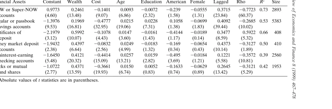
Regression results for NOW or Super-NOW accounts are given in the first row of Table 1. The coefficient of the lagged dependent variable is positively significant and lies within the theoretical bound of 0 and 1. Judging from its magnitude, the average annual speed of adjustment is quite fast; about 63% of the adjustment process would be completed within a year. The short-run wealth and risk-adjusted user cost elasticities are significantly different from 0 at the 5% level. Given the knowledge of the speed of adjustment, the long-run wealth and user cost elasticities are easily computed as 0.39 and 20.22, respectively—approximately 1.59 times larger than their short-run counterparts in absolute terms. Among demographic variables, age and education have significant impacts on asset demand at the 5% level. The t statistics of Rho shows that serial correlation is a problem. The value ofR2is 0.73, which is reasonable
in a two-period cross-sectional analysis.
The second row contains findings on the demand for regular or passbook savings. The short-run elasticities of wealth and risk-adjusted user cost are consistent with economic theories. Age and education are positively related to asset demand, while race and gender have no influence on asset demand. The speed of adjustment can be easily seen to be 0.59, and the long-run coefficient estimates are therefore 1.69 times larger than their short-run counterparts.
Regression results for certificates of deposit show that the short-run coefficients of wealth, risk-adjusted user cost, and age are significantly different from 0 at the 5% level. Given an average annual speed of 0.65, the long-run coefficient estimates are therefore 1.54 times greater than their short-run counterparts in absolute terms.
The results for money market deposits indicate that in the short run a rise in wealth by 100% would raise asset demand by about 44%, while a rise in the risk-adjusted user cost by the same percentage point would reduce asset demand by about 8%. Since the speed of adjustment is 0.56, a rise in wealth by 100% in the long run would raise asset demand by 79%, while a rise in the user cost by 100% would reduce asset demand by 14%. Age again is a significant factor in influencing the demand for these assets in both the short run and the long run.
The short-run demand for non–interest-earning checking accounts are significantly related to wealth and the risk-adjusted user cost at the 5%. Age and education are positively related to asset demand. African-Americans hold less than Whites. Based on the coefficient of the lagged dependent variable, about 88% of the adjustment process would be completed within a year. This means that the absolute values of the long-run coefficient estimates are only 1.14 times greater than their short-run counterparts.
Finally, regression results for stocks and mutual fund shares show that about 74% of the adjustment process could be completed within a year. The long-run coefficients of wealth, user cost, and age are therefore 1.35 time larger than their short-run counterparts in absolute terms.
5. Conclusions
→
Review
of
Economics
and
Finance
8
(1999)
467–478
475
Table 1
Dynamic Demand for Financial Assets by Individuals
Explanatory Variables
User African- Asset Sample
Financial Assets Constant Wealth Cost Age Education American Female Lagged Rho R2 Size
NOW or Super-NOW 0.9773 0.2461 20.1401 0.0093 20.0072 20.239 20.0555 0.3715 20.7723 0.73 2893 accounts (4.60) (13.48) (9.07) (6.86) (2.32) (1.58) (1.31) (23.84) (60.37)
Regular or passbook 21.3976 0.1969 20.4777 0.0215 0.0228 0.1058 20.0699 0.4092 20.2685 0.53 5383 savings accounts (9.53) (16.81) (32.95) (19.06) (7.31) (1.38) (1.83) (39.44) (10.02)
Certificates of 22.1979 0.5992 20.1078 0.0147 20.0161 20.4144 20.0189 0.3477 0.5922 0.66 408 deposit (3.12) (10.07) (4.43) (3.60) (1.43) (1.17) (0.14) (8.59) (5.32)
Money market deposit 21.9432 0.4397 20.0832 0.0249 20.0183 20.169 20.0654 0.4373 20.3127 0.50 410 accounts (2.38) (6.64) (2.56) (4.99) (1.32) (0.34) (0.43) (10.14) (1.89)
Noninterest-earning 21.6450 0.4121 20.4414 0.0257 0.0159 20.495 20.0184 0.1221 20.3572 0.39 2560 checking accounts (5.48) (20.32) (15.09) (13.21) (2.82) (3.69) (1.21) (5.58) (10.81)
Stocks or mutual 21.0722 0.4371 20.3661 0.0150 0.0052 20.1633 20.0629 0.2645 20.3121 0.42 1953 fund shares (2.77) (13.59) (19.93) (6.74) (0.83) (0.74) (0.89) (13.42) (5.29)
speeds of adjustment for major financial assets are fast and within the theoretical bound of 0 and 1. On average, it takes asset holders somewhat more than 1 year but less than 2 years to complete the adjustment process following any disturbance in their socio-economic conditions. In absolute terms, both the short- and long-run coefficients of wealth and user cost for non–interest-earning checking deposits, NOW or Super-NOW accounts, money market deposits, savings deposits, and certificates of deposits are significantly different from 0. Nonetheless, the long-run coefficients are not so large as to cause wide fluctuations in asset demand if socio-economic conditions are disturbed.
Findings in this study have at least three implications. First, these results suggest that many empirical difficulties related to aggregate money demand are probably related to the measurement of monetary aggregates, the identification problem, or the use of proxies. Using microeconomic data that are free from these problems in the short-run money demand models reveals a picture that is quite different from that of aggregate money demand. Second, the impacts of monetary policies on long-run demand for financial assets are not likely to be as large as those suggested in aggregate studies because the speed of adjustment for each monetary asset at the microeconomic level is not as slow as that at the macroeconomic level. Finally, since asset demand is directly related to age in all regressions and influenced by other demographic variables in some regressions, changes in age or other demographic compositions of the population may also have some effects on asset demand in both the short run and the long run.
Acknowledgments
The author is grateful to two anonymous referees for their valuable comments. The views expressed here are solely attributable to the author and are not those of the U.S. Bureau of the Census or the Commerce Department.
Notes
1. Laidler (1977) has a good review of the literature up to the early 1970s, while an excellent survey of the post-1973 literature is provided by Judd and Scadding (1982).
2. In SIPP, longitudinal data are collected in the core modules in which questions on income and program participation are repeated in each wave of a panel, while cross-sectional data are collected in the topical modules only once or twice in a panel. In addition to financial assets, cross-sectional data on health insurance, child care, taxes, migration, and other variables are also collected.
non–interest-earning checking deposits, and the rates of return on these assets are assumed to be 0 in this study.
References
Barnett, W. A. (1980). Economic monetary aggregates: an application of aggregation and index number theory.Journal of Econometrics 14, 11–48.
Barnett, W. A. (1997). Which road leads to stable money demand?The Economic Journal 107, 1171–1185. Barnett, W. A., Offenbacher, E. K., & Spindt, P. A. (1984). The new divisia monetary aggregates.Journal
of Political Economy 96, 1049–1085.
Barnett, W. A., Fisher. D., & Serletis, A. (1992). Consumer theory and the demand for money.Journal of Economic Literature XXX, 2086–2119.
Barnett, W. A., Liu, Y, & Jensen, M. (1997). CAPM risk adjustment for exact aggregation over financial assets.Macroeconomic Dynamics 1, 485–512.
Baumol, W. J. (1952). The transactions demand for cash: an inventory-theoretic approach.Quarterly Journal of Economics 66, 545–556.
Breeden, D. T., Gibbons, M. R., & Litzenberger, R. H. (1989). Empirical tests of the consumption-oriented CAPM.The Journal of Finance 44(2), 231–262.
Chow, G. C. (1966). On the long-run and short-run demand for money.Journal of Political Economy 74, 111–131.
Cooley, T. F., & LeRoy, S. (1981). Identification and estimation of money demand.American Economic Review 71, 825–844.
Friedman, B. M. (1978). Crowding out or crowding in? The economic consequences of financing govern-ment deficits.Brookings Papers on Economic Activity 3, 593–641.
Friedman, M. (1956). The quantity theory of money: a restatement. In M. Friedman (Ed.),Studies in the Quantity Theory of Money(pp. 3–24). Chicago: University of Chicago Press.
Garcia, C., & Pak, S. (1979). Some clues in the case of the missing money.American Economic Review 69, 330–334.
Goldfeld, S. M. (1973). The demand for money revisited.Brookings Papers on Economic Activity, 3, 577–638.
Goldfeld, S. M (1976). The case of the missing money.Brookings Papers on Economic Activity 3, 683–730. Goldfeld, S. M., & Sichel D. E. (1987). Money demand: the effect of inflation and alternative adjustment
mechanisms.The Review of Economics and Statistics 47, 511–515.
Gordon, R. J. (1984). The short-run demand for money: a reconsideration.Journal of Money, Credit, and Banking 16, 403–434.
Hafer R. W., & Thornton, D. L. (1986). Price expectation and the demand for money: a comment. Review of Economics and Statistics 68, 539–542.
Hafer R. W., & Hein, S. (1980). The dynamics and estimation of short-run money demand.Federal Reserve Bank of St. Louis Review 62, 26–35.
Hwang, H. (1985). Test of the adjustment process and linear homogeneity in a stock adjustment model of money demand.The Review of Economics and Statistics 67, 689–692.
Judd, J. P., & Scadding, J. (1982). The search for a stable money demand function: a survey of the post-1973 literature.Journal of Economic Literature 20, 993–1023.
Laidler, D. (1977).The Demand for Money: Theories and Evidence, 2d ed. New York: Harper & Row. Mankiw, N. G., & Shapiro, M. D. (1986). Risk and return: consumption beta versus market beta.Review
of Economics and Statistics 68, 452–459.
Milbourne, R. D. (1983). Price expectations and the demand for money: resolution of a paradox.The Review of Economics and Statistics 63, 633–638.
Theil, H. (1971).Principles of Econometrics.New York: Wiley.
Tobin, J. (1956). The interest elasticity of the transactions demand for cash.The Review of Economics and Statistics 38, 241–247.
Wenninger, J., & Sivesind, C. (1979). Changing the M1 definition: an empirical investigation. Research Paper No. 7904, Federal Reserve Bank of New York.
Appendix
Sources of Income