Simplifying Sirius: sensitivity analysis and development of a
meta-model for wheat yield prediction
Roger J. Brooks
a, Mikhail A. Semenov
b,*, Peter D. Jamieson
caDepartment of Management Science,Management School,Lancaster Uni
6ersity,Lancaster,LA1 4YX,UK bIACR Long Ashton Research Station,Department of Agricultural Sciences,Uni
6ersity of Bristol,Bristol BS41 9AF,UK cNew Zealand Institute for Crop & Food Research Ltd,Pri
6ate Bag4704,Christchurch,New Zealand Received 17 February 2000; received in revised form 19 June 2000; accepted 1 August 2000
Abstract
A sensitivity analysis and analysis of the structure of the Sirius wheat model has resulted in the development of a simpler meta-model, which produced very similar yield predictions to Sirius of potential and water-limited yields at two locations in the UK, Rothamsted and Edinburgh. This greatly increases the understanding of the nature and consequences of the relationships implicit within Sirius. The analysis showed that the response of wheat crops to climate could be explained using a few simple relationships. The meta-model aggregates the three main Sirius components, the calculation of leaf area index, the soil water balance model and the evapotranspiration calculations, into simpler equations. This results in a requirement for calibration of fewer model parameters and means that weather variables can be provided on a monthly rather than a daily time-step, because the meta-model can use cumulative values of weather variables. Consequently the meta-model is a valuable tool for regional impact assessments when detailed input data are usually not available. Because the meta-model was developed from the analysis of Sirius, rather than from statistical fitting of yield to weather data, it should perform well for other locations in Great Britain and with different management scenarios. © 2001 Elsevier Science B.V. All rights reserved.
Keywords:Crop model; Model simplification; Meta-model; Mathematical modelling; Computer simulation
www.elsevier.com/locate/eja
1. Introduction
Process-based models of varying complexity have been developed that can be used to estimate wheat yield at the site scale. These include Sirius
(Jamieson et al., 1998c), AFRCWHEAT2 (Weir et al., 1984; Porter 1993), CERES-Wheat (Ritchie and Otter, 1985), and ECOSYS (Grant, 1998). Each of these is designed to simulate the growth and development of wheat in small, homogeneous areas. They require input data for weather, soil attributes and management practice (choice of cultivar, sowing date, nitrogen application and irrigation) at varying detail. They are able to supply output, on a daily basis, of variables such
* Corresponding author. Tel.:+44-1275-392181; fax:+ 44-1275-394007.
E-mail addresses: [email protected] (R.J. Brooks), [email protected] (M.A. Semenov), [email protected] (P.D. Jamieson).
as biomass, yield, soil water content, mainstem leaf number, leaf area and evapotranspiration. The complexity of the above models, measured as, for example, the number of model parameters, varies substantially. Consequently, the level of input detail also varies substantially. There is a common expectation that the more complex mod-els, because they include explicit descriptions of many sub-processes, should produce more accu-rate results. This is not always so and, in practice, a simple model can predict crop yields as accu-rately as more complex ones (Jamieson et al., 1998b). For example, ECOSYS is a significantly more complex model than Sirius, and requires very detailed input information and high com-puter power to run, but its predictions of grain yield are not better than those from Sirius (Gou-driaan, 1996).
Sirius is a mechanistic model of low to interme-diate complexity, based around a detailed simula-tion of the phenological development of the plant (Jamieson et al., 1998c). The model calculates the final number of leaves using a daylength response mechanism (Brooking et al., 1995; Jamieson et al., 1995a) incorporating a simulation of vernalisation (Brooking, 1996; Robertson et al., 1996), with the number of leaves setting the thermal time to anthesis (Jamieson et al., 1998a). Biomass is accu-mulated according to the amount of light inter-cepted each day, at a light use efficiency that is constant unless reduced by water or nitrogen stress. The simulation of leaf area, which deter-mines the amount of radiation intercepted, and therefore the amount of biomass accumulated, is calculated separately from the number of leaves, although progress after full canopy closure de-pends on phenological development (Jamieson et al., 1998c). Yield is calculated as the biomass accumulated during the grain fill plus up to 25% of the biomass at anthesis. Sirius also includes detailed modelling of the water and nitrogen pro-cesses in the soil as well as transpiration and surface soil evaporation. These are used to deter-mine the amount of water or nitrogen deficit experienced by the plant which can result in re-duced leaf area (hence light interception) and light use efficiency, combining to cause a reduction in the amount of biomass added each day.
Impor-tantly, Sirius has been able to mimic the perfor-mance of wheat crops in experiments in widely different environments over a several-fold yield range (Jamieson et al., 1998b,c, 2000).
In any modelling project, it is important to match the data requirements of the model with the available data and to tailor the process com-plexity to the project objectives (Brooks and To-bias, 1996). For example, excessive detail can lead to a model being inaccurate due to a mismatch of the model and available data. In many regional impact assessments detailed output from the crop models is not required. Instead, information about potential and water-limited yield is usually sufficient. The application of crop simulation models, such as Sirius, requires information on daily weather, soils, and management over a whole region at reasonably high spatial resolu-tion. Such information is often unavailable. A possible solution would be a simplified meta-model with reduced input requirements, but which is able to reproduce the major responses of the original crop model.
so that the model is unrealistic. However, sim-plification of an existing model can give confi-dence in the simplified model by cross-validation against the original more complex model.
The overall aim of the work described here was to develop a simplified meta-model of Sir-ius. The development of the meta-model was carried out in two main stages. Firstly, a tailed sensitivity analysis was carried out as de-scribed in Section 2. This, in itself, gives a better understanding of the responses of Sirius to the input variables and parameters used in the model. Secondly, in order to explain the sensitivity results, the mechanisms of the pro-cesses represented in Sirius were analysed and this analysis is described in Section 3. The meta-model was then based on the simplified relation-ships derived from the analysis of Sirius. The general form of the meta-model is set out in Section 4 along with its specific implementation and the results obtained. Finally, Section 5 dis-cusses the implications of the work.
2. Sensitivity analysis
The ability to be able to aggregate relation-ships into a meta-model depends on the charac-teristics and interactions among the variables in the system being investigated. Therefore, the ini-tial stage of the meta-model methodology was to investigate the relationships between the in-puts and outin-puts of the Sirius model through sensitivity analysis. The sensitivity analysis is de-scribed in this section. A more detailed descrip-tion is given in Brooks and Semenov (1998).
The aim of the sensitivity analysis was to use Sirius to identify which parameters are most im-portant in determining yield. Sensitivity analysis can also act as a verification test by highlighting unusual behaviour, which could be due to er-rors, as well as additional validation in that the relationships observed can be compared with ex-perimental results.
The sensitivity analysis used data for Rotham-sted in the UK, a site where Sirius has been validated (Jamieson and Semenov, 2000) and
where reliable soil data and a long series of weather data were available. Each of the simula-tions was of winter wheat, and, for ease of dis-cussion, the years refer to the year of harvest so that, for example, 1989 refers to wheat sown in autumn 1988 and harvested in summer 1989. The runs were performed in two stages as fol-lows:
1. All of the 20 main Sirius input parameters (Table 1), and the four weather parameters (minimum temperature, maximum tempera-ture, precipitation and radiation) were varied one at a time, in most cases for 51 values over the range 950%. This was done for 2 years; 1989, which is a year with little or no predicted water stress, and a fairly high simulated yield, and 1976, which had extreme summer condi-tions (very hot and dry) resulting in very low simulated yield. Each year was run with nitro-gen limitation turned off, e.g. the nitronitro-gen processes are simulated but the effects of any deficit on the plant are not.
2. In addition to the above scenarios, the weather parameters were varied for each of the years 1961 – 1990 over a more limited range, with nitrogen limitation off, and the results aver-aged in order to obtain an average response to changes in climate.
The base values of the parameters were chosen as typical values for the Rothamsted region or for the UK as a whole. In particular, the sowing date was chosen as 15 October, the cultivar was Avalon, the radiation use efficiency was set at 2.5 g MJ−1, the extinction coefficient was 0.445 and
Table 1
SIRIUS model parameters used for sensitivity tests SIRIUS variable name
Parameter Name Values used at Rothamsted Sensitivity test
range Soil parameters
Saturation soil moisture Qs 44% 925%
0.3
Kq 950%
Reservoir percolation constant
DEF
Initial water deficit 0 0–300
Available and unavailable water AWC[6] and UWC[6], values For AWC: 160; UWC: 80 for the 950% top 25 cm and then 60 for the rest specified for each 25 cm of depth.
capacities
Maximum root depth MaxD 1.5 950%
Vernalisation parameters
VAI
Vernalisation rate response to 0.0012 950%
temperature
0.015
Vernalisation rate at 0°C VBEE 950%
Thermal time parameters
TTSOWEM 150 950%
Thermal time from sowing to emergence
TTANBGF 100
Thermal time from anthesis to 950%
beginning grain fill
TTBGEG
Thermal time from beginning to 650 950%
end of grain fill
90
Phyllochron PHYLL 950%
Culti6ar parameters
Intercept of LAI equation CEPT 2.76 950%
Slope of LAI equation SLOPE 0.00616 950%
8.5
AMNLFNO 950%
Minimum possible leaf no.
AMXLFNO
Maximum possible leaf no. 24 950%
SLDL 0.6 950%
Leaf number daylight response rate
EXTINC
Extinction coefficient (extinction of 0.445 950%
PAR by LAI)
2.5
Radiation use efficiency EFFIC 950%
Soil and cultivar type
7
Soil Types 0–5
Soil type
Cultivar type VARIETY AVALON 14 types
2.1. Summary of sensiti6ity results
2.1.1. Model parameters
Sensitivity analysis using different scenarios may give different results but, based on the runs carried out, the important parameters (in some cases only over certain ranges) out of the 20 input parameters investigated are the initial soil water deficit, the soil depth and available water content, the thermal time parameters for the phyllochron and the grain fill period, the minimum leaf num-ber and the radiation use efficiency (Table 1). Fig. 1 shows the effect of some parameters on simu-lated grain yield for 1989. The base value of the
initial water deficit was zero and this was in-creased up to 300 mm in the sensitivity analysis. The other parameters in Fig. 1 were all varied over the range 950%.
Fig. 1. Sensitivity analysis showing the effect of the most important parameters on yield for Rothamsted 1989 with unlimited nitrogen. The parameters are the initial water deficit (Def), the available water content of the soil layers (Awc), the soil depth (MaxD), the phyllochron (phyll), the grain fill thermal time (bgeg), the minimum leaf number (amnl) and the light use efficiency (par).
parameters determining the growth of the leaf area, those affecting excess water or those that had only a small effect on the anthesis date.
The light use efficiency is a scaling parameter that has the same effect on yield in any scenario, since yield is exactly proportional to the light use efficiency parameter. This parameter is therefore irrelevant in comparing the relative yields between different scenarios such as different soils, culti-vars, sites or climates. To an extent, the thermal duration of the grain fill has a similar effect by scaling the length of the grain fill. The results showed that yield was approximately linearly re-lated to the length of the grain fill period and so it will also often be unimportant in making a comparison of yields. For the Rothamsted cli-mate, the initial water deficit has to be quite large to have any effect. Therefore, in this situation, the only important parameters are the soil depth and available water holding capacity per unit depth for each soil layer (their product across the soil layers is the total soil available water holding capacity, AWC), the phyllochron, and either the minimum leaf number or vernalisation parameters (depending on the choice of cultivar).
The available water content is specified as a soil input parameter in Sirius for each soil layer. The AWC sensitivity factor was applied to the values for all layers. This has a similar effect to applying the same sensitivity factor to the soil depth since, in both cases, the total AWC of the soil will be multiplied by the sensitivity factor (although the water is only available to the plant to the depth of the roots). Yield was found to be approximately linearly related to both factors (and hence to the total soil AWC) in water stressed conditions. For high values of AWC or soil depth, changes in these parameters have less effect because the plant only suffers water stress for part of the period. In 1989, there was sufficient precipitation, for very high values of AWC or soil depth, so that poten-tial yield was reached. At very large soil depths, the roots do not reach the bottom of the soil and so yield is not affected by further increases in soil depth.
Fig. 2. Sensitivity of mean grain yield (a) and its CV (b) simulated by Sirius for 1960 – 1990 at Rothamsted, UK, to changes in temperature, rainfall, radiation and CO2. Precipitation, radiation and CO2were changing by multiplying their values by Factor and
temperature was changing by addingT-factor.
applies to anthesis dates later than the base value (12th June). Consequently, increases in the phyl-lochron in 1989 above the base value tended to decrease yield, with changes in the phyllochron below the base value causing little trend in yield although with some irregular variation. In 1976, the increases in the phyllochron increased yield when the sensitivity factor was less than 1.16.
The minimum leaf number also affects the anthesis date by setting the final number of
leaves although the effect on the anthesis date is less than for the phyllochron. Therefore, the pattern of changes in yield is similar to that for the phyllochron, but of smaller magni-tude.
2.1.2. Weather6ariables
constant sensitivity factors throughout the period. Fig. 2 shows the mean and coefficient of variance of yield for the 30 sensitivity runs for Rothamsted 1961 – 1990.
The response of yield is the most irregular for temperature. The main effect of temperature is to set the phenological dates and so changes in tem-perature affect both the timing and duration of the main growth periods in which most of the biomass is accumulated and during which the water deficit tends to increase. In the runs for both 1976 and 1989, the trend of yield against temperature has maximums at temperature factor values of about −4 and +4 and a minimum in between at about −2°C. The curve of the average values for 1961 – 1990 (Fig. 2a) also has the same pattern, although much less pronounced, and be-tween −2°C and +2°C there is very little change in yield. The sensitivity analysis considers a wide range of temperature variation and the fall in simulated yields for low temperature factors oc-curs because the simulation ceases by default 1 year after the sowing date. In reality, crops ma-turing in October would be at risk from disease. The coefficient of variation for the 1961 – 1990 yields tends to decrease as temperature increases because the earlier maturity means that there are fewer years with a water deficit sufficient to sig-nificantly reduce yield (Fig. 2b). If many years experience a water deficit, differences in precipita-tion mean that the severity of the water deficit varies considerably between years. The difference in yields is therefore much greater than if most years experience no water deficit yield loss.
Changing the precipitation affects the amount of water in the soil and hence the yield loss due to the water deficit. At high precipitation levels, there is sufficient water for the crop and so changes in precipitation have no effect. As with most crop models, there is no disease effect in Sirius and so no penalty for excess water. As precipitation reduces, both the length and severity of the water deficit increase and so each reduction in precipitation causes a progressively larger drop in yield. At very low values, the soil would run out of water during the growing period so that further reductions in precipitation would have less effect. Differences in the water deficit between
different years mean that the coefficient of varia-tion also tends to increase as precipitavaria-tion reduces.
For the lowest values of solar radiation, no water stress is experienced and average yields for 1961 – 1990 initially increase linearly as solar radi-ation is increased. Increased solar radiradi-ation in-creases transpiration and, for each year there is a point after which further radiation increases cause a water stress yield loss. The increasing water deficit results in the average yield reaching a maximum at a radiation factor of about 1.2. The differing water stresses experienced in different years cause the coefficient of variation to increase as radiation increases.
It is assumed that the only effect of an increase in the CO2 concentration is to improve the
effi-ciency of plant photosynthesis. This is imple-mented in Sirius by changing the radiation use efficiency parameter, r, linearly with the increase in CO2 above the baseline value of 353 p.p.m.
Therefore yield is linearly related to CO2, and the
coefficient of variation is constant.
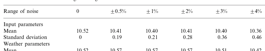
2.2. Random noise
One of the findings of the sensitivity analysis was that a slight change in some of the parame-ters could change the yield by as much as 500 kg ha−1. Any model of this system will inevitably
predic-Table 2
The mean and standard deviation of the yield values (in tha−1) for 1000 sets of parameter values chosen randomly from the
uniform distribution over the given ranges
90.5% 91%
Range of noise 0 92% 93% 94% 95%
Input parameters
10.41
Mean 10.52 10.40 10.41 10.40 10.36 10.32
0.19 0.21 0.28
0 0.36
Standard deviation 0.46 0.57
Weather parameters
10.57 10.57 10.57
10.52 10.51
Mean 10.42 10.32
0.78 0.13 0.22 0.26 0.34 0.39
Standard deviation 0
tion by including excessive detail in crop models. This type of variation is also likely to be present in reality, with yield varying at the field scale due to variations in the quality of both plants and the soil.
The sensitivity of Sirius to small random per-turbations of the input parameters (Table 1) was investigated by running the model for 1989 using random values of the sensitivity factors for each parameter. The factors were obtained by sampling from the uniform distribution over six set ranges from 90.5% up to 95%. Two sets of experi-ments were carried out with the first altering just the input parameters and the second altering just the weather parameters. Each of the weather parameters was varied by applying one factor throughout the period, as before. This represents the effect of a small systematic difference in the values across the whole year, perhaps due to consistent measurement errors or due to the weather site having a slightly different altitude from the field being simulated. The same tempera-ture factor was applied to both minimum and maximum temperature and the range of noise for temperature was based on a typical mean temper-ature value in the growing period of 15°C. For example, for noise of the range91%, the temper-ature factor had the range 90.15°C. For each scenario, the model was run with 1000 sets of parameter values. Table 2 shows the means and standard deviations of yield for each experiment. The results confirm that yield predictions vary significantly for even a small variation in the values of the parameters. The distribution of yield for the input parameter scenarios follows the
nor-mal distribution closely (based on nornor-mal scores plots), except for the 90.5% scenario where there are three distinct distributions resulting from the existence of just three different lengths of grain fill periods. The increase in the variance as the input parameter range increases is approximately expo-nential. For the weather scenarios, the distribu-tion of yield is slightly negatively skewed. The actual yield value for the base parameter values (10 521 kg/ha−1) is just a single point and the
mean values for small random noise in the parameters (:10 400 kg/ha−1
) would therefore be a more appropriate result for this scenario.
The variation in yields for small changes in the parameters sets a limit on the match with ob-served yields that is possible with such a simula-tion model. Because similar random variasimula-tions are likely to be present in the observed values, a perfect match between observed and simulated yields should not be expected. Tests of models should therefore use yields over a wide range so that the differences in yields are mainly due to differences in conditions for each scenario rather than local random variation (Jamieson et al., 1999).
3. Simplifying Sirius equations
3.1. Yield equation
The biomass added each day by Sirius through-out the simulated growth of the plant is given in gm−2 by
biomass added in one day=0.48Srb(1−e−xl)
(1)
where S is the global solar radiation for the day (MJ m−2), 0.48 is a transfer coefficient between
global radiation and photosynthetically active ra-diation (PAR), r is the light (or radiation) use efficiency (g MJ−1
), b(05b51) is the reduction factor for the light use efficiency due to drought,
xis the extinction coefficient andlis the leaf area index (LAI). The term 0.48S(1−e−xl) represents
the amount of PAR intercepted by the plant. Asl
increases, the radiation intercepted, and hence the biomass, increasess but the rate of increase be-comes less due to the fact that new leaves will tend to overlap existing leaves. In particular, un-less the leaf area is small, the biomass added is not sensitive to changes in the leaf area index.
In the grain fill period (GFP) all the biomass accumulated is allocated to the grain. The leaf area is reduced proportionally to the square of accumulated thermal time, although the daily thermal time value used is multiplied by a water deficit factor,k(15k51.5). The equation for leaf area, l, during grain fill is
l=L
1−(kTacc)2
TGFP
2
(2)whereLis the LAI at the start of grain fill,Taccis the accumulated thermal time to date in grain fill and TGFP is grain fill period thermal time. The grain fill period ends when the leaf area reduces to zero. In the absence of a water deficit the thermal time of grain fill will therefore be TGFP, but the thermal time will be reduced if such a deficit causes k to be greater than one. At anthesis the LAI will be at a value of 8.5 (a fixed Sirius parameter), unless a water deficit before anthesis reduces this value (although a severe deficit is required for a significant reduction). The LAI will reduce slightly in the few days between anthesis and the start of grain fill so thatLwill usually be between 8 and 8.5.
In the analysis, constant values for b, k, Sand the daily thermal time T will be assumed during the grain fill period. Then, by substituting Eq. (2) for the reducing leaf area index into Eq. (1) and integrating over the grain fill period, the biomass added during the grain fill period is given by
GFP biomass=
&
TGFP
The division by T converts the daily biomass of Eq. (1) into biomass per unit thermal time. This is then integrated over the grain fill period thermal time. Strictly, this relationship is modelled in Sir-ius just at the daily time step rather than continu-ously. In addition, a drought deficit during the few days between anthesis and the beginning of grain fill slightly reduces the length of the grain fill period in Sirius, although this effect is small and has been ignored in Eq. (3).
The integral can be evaluated by expanding the Taylor series for the exponential function and then integrating term by term (Ferrar, 1980 p114 Theorem 46) to give
GFP biomass=0.48SrbTGFP
kT
period in days. The term within the outer brackets is the average proportion of radiation intercepted over the grain fill period. We will denote this by
f(x,L). This term can be evaluated easily but a good approximation (over the range of usual x
values) is also given by 1−e−xL
unlessLis very small, the value will be close to 1. As for the daily biomass equation, f(x,L) is not particularly sensitive to the value ofLunlessLis small. For example, here x=0.445 and L values of 6, 7 and 8 givef(x,L) values of 0.76, 0.80 and 0.83 respectively.In Eq. (4), r, TGFP and x are cultivar
about 8 and, in any case, the GFP biomass is not sensitive to this value. GFP biomass therefore mainly depends on the photothermal quotientS/
Tduring grain fill and the water deficit variablesb
and k. The photothermal quotient will be deter-mined by the weather pattern in the particular year and the specific timing of the grain fill period.
The final yield is the sum of the biomass added in the grain fill period and a proportion (up to a maximum of 0.25) of the anthesis biomass,A. The anthesis biomass is added to the yield over the grain fill period with the amount added each day being 0.25A×T/TGFP. However, since the num-ber of days of the grain fill period isTGFP/kT, the total anthesis biomass included in the yield will be 0.25A/k. Again, the slight reduction in the length of the grain fill period due to a drought between anthesis and the start of grain fill has been ig-nored. Therefore, the yield is given in gm−2 by
yield=1
k
0.25A+4.8SrbTGFP
T f(x,L)
(5)The anthesis biomass consists of the accumulation of biomass from the emergence of the plant until anthesis. The biomass added each day is given by Eq. (1). The total biomass accumulated therefore depends on the length of this period, which is set in thermal time, as a number of phyllochrons, by the calculation of the final number of leaves (which uses vernalisation and input cultivar leaf parameters). The phyllochron is also a cultivar parameter input by the user. After emergence the LAI increases from zero as a function of thermal time, although the initial increase is rapid and so the biomass added soon becomes insensitive to the precise LAI value. For a given thermal time period from emergence to anthesis, the total biomass accumulated depends on the rate of in-crease of biomass per unit of thermal time. The biomass added is proportional to solar radiation,
S, and so, as for GFP biomass, anthesis biomass depends on the weather through the values of the photothermal quotient. The values during the ini-tial part of the period when LAI is small are the least important.
As for the grain fill period, a water deficit prior to anthesis can reduce the biomass through a light
use efficiency factor and can reduce the LAI. However, the deficit has to be very large for a direct reduction of biomass to occur, which is very unlikely in the UK. As already discussed, reductions in the LAI have little effect on the biomass added unless the LAI becomes very small which again is unlikely in the UK. Any effect is further reduced by the fact that at most one quarter of the anthesis biomass is included in yield. In Sirius, a drought deficit prior to anthesis has no effect on the timing of phenological events. Therefore, no effect of a water deficit prior to anthesis has been included in the yield equation.
The effect of the water deficit factor can be seen by denoting the potential grain fill biomass byG, where
G=4.8SrTGFP
T f(x,L). (6)
Therefore, the potential yield is 0.25A+G com-pared to the actual yield of (0.25A+bG)/k. The maximum value ofkin Sirius is 1.5 and so it can reduce yield by up to one third. The light use drought factor, b, takes values between 0 and 1. Interestingly, this linear model of grain yield re-duction in drought is conceptually similar to the Penman (1971) drought response model, tested successfully for wheat and other crops by Jamieson et al. (1995b).
The next sub-section explains the water balance and the calculation of the water deficit factors in Sirius.
3.2. Water balance and deficit
amount transpired=PTAY×WSF
×(1−e−xl) mm day-1 (7)
where WSF is a water deficit stress factor and PTAY is the Priestley – Taylor function (Priestley and Taylor, 1972), given by
PTAY=1.5 H
H+0.66(0.241S−0.1) mm day
-1
(8)
where H is the slope of the saturated vapour pressure temperature curve (hPa °C−1). Based on
typical values of H in the summer months at Rothamsted,
PTAY:0.19S mm day-1
. (9)
During most of the growth period the leaf area is not small and so 1−e−xl:1. Therefore, during
this period,
amount transpired:0.19×S×WSF mm day -1.
(10)
During the winter months the only effect is the addition of precipitation to the soil. In the UK climate this often leaves the soil fully saturated. A water deficit will therefore only accumulate during the main growth period once the amount tran-spired starts to exceed the average precipitation level. The daily amount of water removed from the soil will then be given by
water removed:0.19×S×WSF−P mm day-1
(11)
whereP is the precipitation in mm that day. The water deficit, D, experienced by the plant there-fore mainly depends on the values of solar radia-tion and precipitaradia-tion in the growth period.
If the useable water in the root zone of the plant is at least half the available water capacity, the water stress factor, WSF, equals one (i.e. no effect). Otherwise the water stress factor is twice the useable water divided by the available water capacity, AWC. Since the useable water is the AWC−water deficit, the water stress factor is
WSF=min
2(AWC−D)AWC ,1
(12)Therefore, the water deficit on day t, Dt, can be estimated by the recurrence relation
Dt=max
Dt−1+0.19×St×min
2(AWC−Dt−1)AWC ,1
−Pt,0 (13)where St and Pt are the solar radiation and pre-cipitation on dayt. This relationship was found to model the water deficit well whether using actual daily values for the weather variables or using the average values for the month.
A water deficit can affect the biomass or LAI in Sirius through water deficit factors. In addition to the grain fill factors b and k explained above, there are also LAI and biomass factors prior to anthesis. These factors are all linear functions of
WSF within certain ranges of WSF. For example
k=1 for WSF]0.7, k=1.5 for WSF50.4 and
k=21/
6−5WSF/3 for 0.45WSF50.7. In
particu-lar, for a given water deficit, the Sirius water deficit factors can be calculated easily. Since WSF
is also linearly related to the water deficit, D, the factors are also linearly related to the water deficit. The light use factor, b, is given by b=
min(2WSF,1) and so only has an effect when
WSFB0.5, i.e. when the useable water is less than 1/4 AWC.
3.3. Explanation of the sensiti6ity results
The sensitivity results can be explained using the analysis of the model already set out. A full explanation is given in Brooks and Semenov (1998). For unlimited nitrogen, the analysis indi-cates that yield should be approximately given by Eq. (5) with the drought factors depending on the water balance as given above. For example, in the sensitivity analysis, yield was exactly proportional to the light use efficiency, r. This is because both the grain fill period and anthesis biomass are proportional tor, andrhas no effect on the water balance. In the sensitivity results, yield is not very sensitive to the extinction coefficient, x, although the relationship does approximately follow a 1
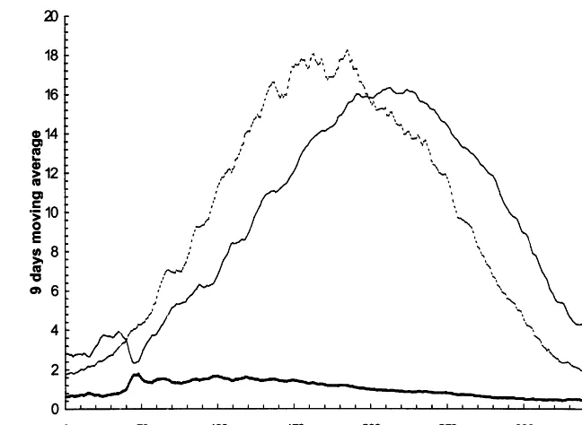
Fig. 3. Nine days moving average of temperature, radiation and photothermal quotient at Rothamsted for average 1961 – 1990 weather data.
Several parameters in the model affect the an-thesis date. Changing the anan-thesis date alters the anthesis biomass by changing the timing and length of the growing period up to anthesis and, just as important, alters the timing of the grain fill period. A change in timing will also alter the water deficit experienced during the grain fill pe-riod. A change in anthesis date by a few days will alter the yield in an irregular manner depending mainly on differences in weather on the days that are added or removed from the grain fill period. A large change in anthesis date is likely to cause an overall trend in yield in addition to the irregular changes.
Anthesis date is mainly determined in Sirius by the number of leaves and the phyllochron, which determine the length of the thermal time period from emergence to anthesis. Extending this period will increase the anthesis biomass. The resulting change in the timing of the grain fill period also changes the grain fill biomass due to different values for the water deficit and the photothermal quotient,S/T, during the grain fill period. For the dry year of 1976, a delay in anthesis date tends to
reduce the yield because the water deficit builds up over a longer period and the greater yield loss due to the increased water deficit has more effect on yield than the increase in anthesis biomass. Yield does increase again for a large delay be-cause the grain fill period is moved into the middle of July when there were a couple of weeks with a significant amount of precipitation. A de-lay in the anthesis date for 1989 from the base value also tends to decrease yield for the same reason (Fig. 1). Using the base parameter values, the anthesis dates in 1976 and 1989 were 15th and 12th June, respectively. In both years, the pho-tothermal quotient tends to reach a maximum towards the end of April and decline thereafter and so a delay in the anthesis date also tends to reduce the potential grain fill period biomass.
through-out the year but it will also make the phenological dates earlier (in particular the anthesis date and the grain fill period), since the phenological peri-ods are specified in thermal time. The reduction in
S/Treduces the potential anthesis biomass. How-ever, an earlier grain fill period means thatS/Tis closer to its maximum value during the grain fill period (Fig. 3) and so there is much less change in the value ofS/Tduring the grain fill period and, hence, in the potential grain fill period biomass. An earlier grain fill period also reduces the water deficit during the grain fill since the deficit builds up over a shorter period of time. The interaction of these factors produces the complex response of yield, together with the limit of 1 year for the simulated period explained in Section 2.1. In par-ticular, yield is roughly constant within the range 92°C.
Changes in radiation and precipitation, on the other hand, have a negligible effect on key devel-opment dates. An increase in radiation increases the rate of accumulation of biomass throughout the year and increases the water deficit through greater transpiration by the plant. For low values of solar radiation, the water deficit is small enough that the potential yield is obtained. Both potential anthesis biomass and potential grain fill biomass are proportional to solar radiation and so the yield is also proportional. Apart from the feedback effect of the stress factor, the water deficit is also linearly related to radiation (Eq. (13)), and the deficit factors b and k are linearly related to the deficit. As a water deficit increases, at first the yield is reduced by the effect ofk and then, for a more severe deficit, by the effect ofb. Initially, increases in a deficit both reduce k and increase the proportion of the grain fill period it affects. This results in the curve in the high solar radiation values in Fig. 1. Precipitation affects only the water deficit and its values are similarly curved. The results for 1976 and 1989 show that, for low water values,kceases to have any further effect (if WSFB0.4) and so the curve would tend to flatten out. Below this yield is approximately linearly related to precipitation through the effect of b.
4. Meta-model
4.1. Conceptual model
Based on the analysis described above, a sim-plified meta-model was developed assuming un-limited nitrogen. The meta-model is based on the yield Eq. (5) and the simplified water balance given by Eq. (13). Eq. (5) also requires the anthe-sis date and the antheanthe-sis biomass.
The meta-model consists of seven steps, but these can be implemented at several different lev-els of detail. The steps together with the alterna-tive methods that could be used for each step are as follows:
Step1. Calculate the final leaf number. The full Sirius mechanisms of vernalisation and the leaf number calculation, using thermal time and daylength could be used for this step. However, for similar conditions such as different years at the same site, it appears that final leaf number is approximately linearly related to mean tem-perature over the winter period and so a regres-sion equation fitted to Sirius output could be used.
Step 2. Calculate the anthesis date. The total thermal time from sowing to anthesis is fixed once the leaf number is known. Sirius assumes 0.75 phyllochrons for each of the first two leaves, one phyllochron for each of the next six leaves and 1.3 phyllochrons for each additional leaf. The anthesis date can be calculated using temperature data as the date at which the ther-mal time to anthesis is reached.
Step3. Calculate the potential anthesis biomass
A (which equals actual anthesis biomass since anthesis biomass is affected very little by water stress). This depends mainly on the photother-mal quotient, S/T, in the main growing period up to anthesis (typically, in the UK, about 3 months). The analysis indicates that an approx-imately linear relationship should exist between yield and the average value of S/T for the period before the anthesis date for UK condi-tions. This should enable a regression equation to be fitted to Sirius output.
the average value of S/T for the grain fill period. In most circumstances, a value of about eight will be suitable for the leaf area at the start of the grain fill, L. The grain fill period can be identified using temperature data to accumulate thermal time, and using the input thermal time values from anthesis to the start of the grain fill and from the start to the end of the grain fill. If preferred, the last few days of the grain fill period can be ignored in calculat-ing the average since these are the least impor-tant for accumulating biomass.
Step5. Calculate the potential yield as 0.25A+
G.
Step 6. Calculate the water deficit during the grain fill period by accumulating the deficit using Eq. (13) and values of solar radiation and precipitation. Alternatively, it may be possible to fit a regression equation to Sirius output relating the water deficit to the accumulated value of 0.19S−P over the period from when this starts to take positive values until the mid-dle of the grain fill period.
Step7. Calculate the average of the water stress factors b and k during the grain fill period. These are simple linear functions of the water deficit. The simplest way to do this is to use the water deficit calculated for the middle of the grain fill period. A more precise method is to calculate daily values for the factors during the grain fill using the water deficit from step 6 and then take an average. If the water deficit is very high, the grain fill period will be shortened to a length of TGFP/k, and so a revised grain fill period can be calculated using an average k
value. Then the average of the drought factors can be calculated just over the revised period. If necessary, a revised value of G can also be calculated using this revised period (step 4).
Step 8. Calculate the final yield as 1
k(0.25A+ bG).
Where weather data is used, either daily data or disaggregated monthly data (where the average value for the month is assigned to each day) could be used. The fact that yield can be related to cumulative values indicates that using monthly weather data should give similar results to using daily weather data.
Whichever way the meta-model is implemented, the main differences from Sirius are the absence of three of the principal Sirius model components, namely the model of leaf area index, the soil water balance model, and the evapotranspiration calcu-lations. In addition, the growth of the plant is not simulated on a daily basis but, rather, biomass is related to the accumulated weather variables. In-deed, the only daily calculations are the adding up of the weather variables. An important character-istic of the meta-model is that it contains very little interaction between the components. Once the anthesis date and leaf number are known, the anthesis biomass, the GFP potential biomass and the water stress yield loss are all calculated sepa-rately. The meta-model also calculates both po-tential and water limited yield in one run.
The meta-model does not require the leaf area to be simulated but, instead, just uses average values of the photothermal quotient, S/T. The relationship between biomass and S/T exists be-cause the pattern of change in leaf area will tend to be similar across different scenarios and be-cause, in the UK, the biomass added is not sensi-tive to changes in leaf area.
The important variable for water stress is the water deficit during grain fill. This can be mod-elled well using Eq. (13) rather than with a de-tailed model of the soil in layers and the dede-tailed evapotranspiration calculations.
4.2. Meta-model implementation and results
A meta-model was coded in Borland C++
Builder for Windows 9× /NT/2000 following the conceptual model1. Where there was a choice of
methods to use, the model was constructed so as to be generally applicable for a wide range of circumstances.
The calculation of final leaf number uses the full Sirius daylength response mechanism so that it can be used for different varieties, latitudes and sowing dates. The ratio of total radiation for the 90 days prior to anthesis divided by total thermal time for that 90 days is used to calculate the
1Meta-model is available from www.lars.bbsrc.ac.uk/model/
anthesis biomass using a regression relationship fitted to the Sirius Rothamsted output data for Rothamsted for 1961 – 1990 with precipitation multiplied by 0.5 (to make all yields water lim-ited). The regression relationship had a coefficient of determinationR2 value of 0.83.
The same ratio is calculated for the grain fill period (with the period being determined by accu-mulating thermal time after anthesis) and the grain fill period biomass calculated using the Eq. (2). The potential yield is then given by the grain fill period biomass plus one quarter of the anthe-sis biomass.
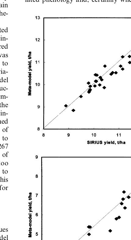
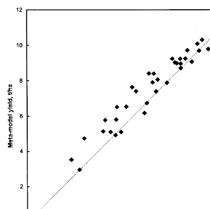
The meta-model was run for Rothamsted 1961 – 1990 with 50% precipitation and for Edin-burgh with a poor soil and the results compared with those from Sirius. Daily weather data was used in both cases. The scenarios were chosen to give a wide range of yields mainly due to varia-tions in water stress. Fig. 4 shows meta-model yield versus Sirius yield for (a) potential produc-tion and (b) water limited producproduc-tion at Rotham-sted. Fig. 5 shows the meta-model yield versus the Sirius yield for water limited production at Edin-burgh. In both cases the meta-model performed well giving a root mean square error (RMSE) of 682 and 831 kg/ha−1
respectively (compared to the standard deviations in Sirius yields of 1267 and 2176 kg/ha−1) and correlation coefficients of
0.92 and 0.95. The leaf number tended to be too low for Rothamsted by about 0.4 leaves due to Sirius using soil temperature and correcting this by adding 0.4 leaves reduced the RMSE value for Rothamsted to 457.
4.3. Implications of the meta-model results
The good match of the meta-model yield values with those of Sirius indicates that the meta-model does contain the important aspects of Sirius and, in particular, that there are no other Sirius mech-anisms substantially affecting the yield. Because the meta-model is based on analysis of the Sirius model, rather than just on its output, it should be able to match the Sirius output well for most scenarios in Britain (e.g., different sowing dates or cultivars) and probably for many other climates without serious modifications. The approximation
of the Priestley – Taylor function PTAY in Eq. (9) will probably need an adjustment for a dry and hot climate. An effect of pre-anthesis drought
may also need to be included in such
circumstances.
The fact that the meta-model can reproduce the Sirius yield well does not necessarily mean that it should be used instead of Sirius. Sirius is a generic, mechanistic model with a detailed simu-lated phenology and, certainly where detailed
Fig. 5. Yield simulated by the meta-model versus yield simu-lated by Sirius at Edinburgh for 1960 – 1990 and poor soil (0.5 m) for water-limited production.
lochron). Solar radiation affects not only poten-tial yield but also the water deficit. However, this variable is often not directly measured but must be estimated from some other variable such as sunshine hours, for example. This makes its value uncertain and it is therefore important that sensi-tivity analysis is carried out on this variable.
The meta-model uses average or accumulated values of the weather variables and is able to perform well just with monthly weather data. It was run at Rothamsted with 50% precipitation and at Edinburgh for the soil with low AWC (80 mm), using daily weather data and 30-day moving average weather data. RMSE for the anthesis day and water-limited yield are 1 day and 147 kg/
ha−1
, and 1.7 days and 470 kg/ha−1
for Rotham-sted and Edinburgh, respectively. This indicates that replacing daily data with disaggregated monthly data in Sirius is unlikely to change the output significantly.
The meta-model identifies a further way of comparing Sirius with experimental data since the derived relationships should be present in the experimental data if Sirius is performing well. Parts of the model could also form the basis for further model development. Perhaps the pho-tothermal quotient could have significance in terms of the physical processes of the plant but a more likely path would be to use the relationship of yield loss to 0.19S−P as a basis for simpler modelling of water stress.
5. Summary and conclusions
The sensitivity analysis and the further analysis of Sirius identified the parameters and variables that are the most important for model calibration and performance. For example, the total available water capacity is the most important soil parame-ter. This allows different soil types to be grouped together for regional impact assessments (Brooks and Semenov, 2000). The interesting responses of the simulated grain yield to mean temperature changes at Rothamsted have potential implica-tions for climate change studies. When the mean temperature increases, the photothermal quotient put data is available, it is likely to give more
phyl-decreases resulting in a decrease in total biomass and grain yield (Wolf et al., 1996), except where crop growth is limited by water stress. Then the shortening of the growth period reduces the ex-posure to water stress. The compensating effect of these factors means that, at Rothamsted, sim-ulated grain yield shows little variation between temperature changes −2°C and 2°C.
The sensitivity analysis also found pseudoran-dom variations in simulated grain yield (up to 500 kg ha−1) as a result of slight changes (up
to 5%) in some model parameters and input variables. These cannot be determined precisely, which sets a limit to the accuracy of the yield prediction. This needs to be accounted for when comparing simulated and observed yield.
The development of a relatively simple meta-model greatly increases the understanding of the consequences of the relationships implicit within Sirius and shows, in particular, that the re-sponse to climate can be explained using a few simple relationships. Aspects of Sirius left out of the meta-model are the calculation of the leaf area index, the soil water balance model and the evapotranspiration calculations. The meta-model essentially uses cumulative values of weather variables, indicating that disaggregated monthly values should produce similar results in Sirius to those using daily weather data. The faster run time of the meta-model and the ability to analyse its results more easily may make it a valuable tool for regional impact assessments when many runs are required. Its level of detail may also be more appropriate in such circum-stances since detailed high-resolution input data are usually not available.
The meta-model has mimicked well potential and water – limited yields simulated by Sirius at
two locations, Rothamsted and Edinburgh.
Since the meta-model was developed from the analysis of Sirius, rather then from statistical fitting of output data, it should perform well for other locations in Britain and different manage-ment scenarios. It is likely that the meta-model will match Sirius yield well for diverse environ-ments and climates without serious modifica-tions, but this hypothesis needs further testing.
Acknowledgements
Weather datasets were supplied by the UK Meteorological Office through the Climate Im-pacts LINK project and the ARCMET data-base. The work of R.J.B. was supported by the
European Commission’s Environment
Pro-gramme under Contract Number ENV4-CT95-0154. IACR Long Ashton receives grant-aided support from the Biotechnology and Biological Sciences Research Council of the United King-dom.
References
Brooking, I.R., 1996. The temperature response of vernaliza-tion in wheat-a developmental analysis. Ann. Bot. 78, 507 – 512.
Brooking, I.R., Jamieson, P.D., Porter, J.R., 1995. The influ-ence of daylength on the final leaf number in spring wheat. Field Crops Res. 41, 155 – 165.
Brooks, R.J. and Semenov, M.A. 1998. Sensitivity analysis of the Sirius wheat model, Technical Report, IACR Long Ashton Research Station.
Brooks, R.J., Semenov, M.A., 2000. Modelling climate change impacts on wheat in central England. In: Climate Change, Climatic Variability and Agriculture in Europe. An Inte-grated Assessment. Downing, T.E., Harrison, P.A., But-terfield, R.E., Lonsdale, K.G. (Eds.), Research Report No. 21, Environmental Change Unit, University of Oxford, Oxford, pp. 157 – 178.
Brooks, R.J., Tobias, A.M., 1996. Choosing the best model: Level of detail, complexity and model performance. Math. Comp. Modelling 24 (4), 1 – 14.
Brooks, R.J., Tobias, A.M., 1999. Methods and benefits of simplification in simulation. In: Al-Dabass, D., Cheng, R.C.H. (Eds.), UKSim 99 Fourth National Conference of the U.K. Simulation Society, 7 – 9 April 1999. UK Simula-tion Society, St Catharines College, Cambridge, pp. 88 – 92. Ferrar, W.L., 1980. A Textbook of Convergence. Oxford
University Press, Oxford.
Goudriaan, J., 1996. Predicting crop yields under climate change. In: Walker, B.H., Steffen, W. (Eds.), Global Change and Terrestrial Ecosystems. Cambridge University Press, Cambridge, pp. 260 – 274.
Grant, R.F., 1998. Mathematical modelling of root growth under different nitrogen and irrigation treatments: the ecosys approach. Ecol. Modelling 107, 237 – 264. Jamieson, P.D., Brooking, I.R., Porter, J.R., Wilson, D.R.,
1995a. Prediction of leaf appearance in wheat: a question of temperature. Field Crops Res. 41, 35 – 44.
Jamieson, P.D., Brooking, I.R., Semenov, M.A., Porter, J.R., 1998a. Making sense of wheat development: a critique of methodology. Field Crops Res. 55, 117 – 127.
Jamieson, P.D., Porter, J.R., Goudriaan, J., Ritchie, J.T., Keulen, H., van Stol, W., 1998b. A comparison of the models AFRCWHEAT2, CERES-Wheat, Sirius, SU-CROS2 and SWHEAT with measurements from wheat grown under drought. Field Crops Res. 55, 23 – 44. Jamieson, P.D., Semenov, M.A., Brooking, I.R., Francis,
G.S., 1998c. Sirius: a mechanistic model of wheat response to environmental variation. Eur. J. Agron. 8, 161 – 179. Jamieson, P.D., Porter, J.R., Semenov, M.A., Brooks, R.J.,
Ewert, F., Ritchie, J.T., 1999. Comments on ‘‘Testing winter wheat simulation models’ predictions against ob-served UK grain yields’’ by S. Landau et al (1998). Agric. For. Meteorol. 96, 157 – 161.
Jamieson, P.D.; Berntsen, J.; Ewert, F.; Kimball, B.A.; Olesen, J.E.; Pinter, P.J.; Jr, Porter, J.R.; Semenov, M.A.; 2000. Modelling CO2 effects on wheat with varying nitrogen
supplies, Agro-Ecosystems and Environment (in press) Jamieson, P.D., Semenov, M.A.; 2000. Modelling nitrogen
uptake and redistribution in wheat, Field Crops Res. (in press)
Penman, H.L., 1971. Irrigation at Woburn VII. Report Rothamsted Experimental Station for 1970 2, 147 – 170. Porter, J.R., 1993. AFRCWHEAT2: a model of the growth
and development of wheat incorporating responses to wa-ter and nitrogen. Eur. J. Agron. 2, 69 – 82.
Priestley, C.H.B., Taylor, R.J., 1972. On the assessment of surface heat flux and evaporation using large scale parame-ters. Monthly Weather Review 100, 81 – 92.
Ritchie, J.T., Otter, S., 1985. Description and performance of CERES-Wheat: A user-oriented wheat yield model. In: Willis, W.O. (Ed.), ARS Wheat Yield Project, Department of Agriculture, Agricultural Research Service, ARS 38, pp. 159 – 175.
Robertson, M.J., Brooking, I.R., Ritchie, J.T., 1996. The temperature response of vernalization in wheat: modelling the effect on the final number of mainstem leaves. Ann. Bot. 78, 371 – 381.
Weir, A.H., Bragg, P.L., Porter, J.R., Rayner, J.H., 1984. A winter wheat crop simulation model without water or nutrient limitations. J. Agric. Sci. Camb. 102, 371 – 382. Wolf, J., Evans, L.G., Semenov, M.A., Eckersten, H., Iglesias,
A., 1996. Comparison of wheat simulation models under climate change. I. Model calibration and sensitivity analy-ses. Climate Res. 7 (3), 253 – 270.