Vol. 42 (2000) 207–229
An experimental examination of double marginalization
and vertical relationships
Yvonne Durham
∗Department of Economics, College of Business Administration, 402 Business Administration Bldg., University of Arkansas, Fayetteville, AR 72701, USA
Received 5 January 1998; received in revised form 6 October 1999; accepted 15 December 1999
Abstract
The presence of a vertical externality, and therefore an incentive to integrate or to impose vertical restraints, is investigated in 11 posted-offer experiments. Upstream markets are characterized by a single seller. When the downstream market consists of three firms, there is no evidence of a vertical externality, and behavior is consistent with the vertically integrated outcome. With a single firm downstream, a vertical externality is present and the Nash prediction is supported. An analysis of individual market behavior reveals that firms approximate their best response functions, with some indication that they improve over time. © 2000 Elsevier Science B.V. All rights reserved.
JEL classification: L1; D4
Keywords: Double marginalization; Experiments; Monopoly; Vertical restraints; Vertical integration
1. Introduction
Vertical relationships among firms have been of continuing interest to industrial orga-nization economists and antitrust authorities. Although the relationship between upstream firms and downstream firms is in some ways similar to the relationship between a firm and its customers, a vertical relationship between firms can be more complex. In a vertical structure, some decisions, such as the final price, the amount of services, the promotional effort, are made after the intermediate good is sold by the upstream firm and are therefore no longer in its control. Since these additional decisions affect the upstream firm’s profit, an upstream firm may have an incentive to attempt to control them. The maximum profit that can be earned by the vertical structure is the integrated profit — or the profit that an integrated firm, controlling all the decisions made by the structure, could earn. Much of
∗Fax:+1-501-575-7687.
the literature in this area has focused on the issue of vertical control and the set of vertical restraints sufficient for the vertical structure to obtain the integrated profit.
Incentives to integrate or to impose vertical restraints can come from a variety of sources. The market power incentive, or the incentive which arises when the downstream market is not competitive, comes from this inability of the upstream firm to control downstream decisions.1 A monopoly producer of an intermediate good will charge its downstream customers a price which is greater than its marginal cost. If the downstream market is not competitive, specifically if it is also monopolized, then the price of the final good will also be marked up above its cost. Each time the downstream firm takes any action to increase the quantity it sells (i.e., lowers price, increases promotional effort), the upstream firm’s profit is increased. However, the downstream firm does not take this into account when it makes its decision and therefore tends to restrict quantity relative to the vertically integrated solution. This is referred to as the vertical externality and provides an incentive for the imposition of vertical restraints by the firm upstream.
A well-known illustration of this basic externality is due to Spengler (1950). He uses a fairly simple model to examine the increase in efficiency that occurs with vertical integration when the downstream market is monopolized. In his model, the downstream firm’s only de-cision is the retail price. When both the upstream and downstream markets are monopolized, the presence of the vertical externality causes the final price to be higher and the aggregate profits to be lower than if the firms were vertically integrated. The upstream firm charges a price higher than its marginal cost, causing the cost facing the downstream firm to be higher than the vertical structure’s cost. The downstream firm then behaves as a monopolist with this marginal cost and prices above it. Therefore, two successive markups occur, creating a ‘double marginalization’ problem. The distortion caused by the downstream monopolist lowers upstream profits. This provides the upstream firm with an incentive to attempt to control downstream actions. The vertical structure earns lower aggregate profits and con-sumers are worse off because of the quantity decrease and price increase. In this simple environment, vertical integration improves the efficiency of the market.
If the downstream market is competitive, this vertical externality is eliminated, and the fi-nal outcome is identical to the vertically integrated outcome. The fifi-nal price is forced down to the downstream marginal cost and the structure earns the vertically integrated profit. Competition in the downstream market effectively controls price for the upstream monop-olist. Welfare is enhanced and aggregate profits are increased. The incentive to vertically integrate or impose restraints is removed in this case.
Vertical relationships among firms as such are not well explored in the experimental economics literature. Because this particular theory is basic to much of the work done in the vertical restraints and control area, its performance in a controlled laboratory setting has important implications. If the presence of market power in the downstream market does not create a vertical externality, the incentive to integrate must come from different sources. The purpose of the experiments reported here is to provide an initial test of Spengler’s model (as described in Tirole (1988)). If we find, as theory predicts, that the vertical externality is present in experimental markets with monopoly power at both stages of production and
1We will ignore other incentives for integration such as the elimination of transaction costs or the realization of
that the externality disappears when competition is introduced in the downstream market, the argument for allowing vertical integration into non-competitive downstream markets to improve efficiency will be supported, since the vertically integrated outcome is theoretically identical to the outcome when there is competition downstream.
Although we have discussed three different types of vertical market structures here — monopoly/monopoly, monopoly/competition, and a vertically integrated monopoly, the ex-periments discussed here examine only the first two since the behavior of monopolists in simple posted offer markets has been well-documented (see Smith (1981); Harrison and McKee (1985); Harrison et al. (1989) among others). Posted offer monopolists with full information, facing simulated buyers and constant costs have been found to have the most success at exploiting their monopoly power. In both structures examined in these exper-iments, the upstream market consists of a single seller. In one structure, the downstream market is characterized by a single seller, while competition, in the form of three sellers, is introduced in the other.
Previous experimental work has studied problems of a similar nature, but in different contexts. Interdependent markets have been the basis of a number of studies. Miller et al. (1977), Williams (1979), Hoffman and Plott (1981) and Williams and Smith (1984) all ex-amine the effects of the introduction of intertemporal speculators into markets with cyclical demand and/or supply, using either the double auction or the posted offer institution. The speculators in these experiments were faced with a similar problem to that of a downstream firm. The intertemporal competitive equilibrium price and quantity were generally sup-ported, and the presence of speculators increased efficiency in these markets. In all cases, two to four speculators were used.
In a similar setting, Plott and Uhl (1981) investigated the role of middlemen in dou-ble auction markets. Some subjects, known as traders, first participated as the buyers in one market with other subjects who were sellers. The traders then became the sellers of those units in another market with a set of subjects who were designated as buyers. The upstream firm, downstream firm, and final buyers scenario could easily be applied to these experiments. The competitive solution was supported with the middlemen present, and contrary to popular belief, the middlemen did not profit at the expense of the buy-ers and sellbuy-ers. In all cases, three or four tradbuy-ers were used. None of the middlemen or speculator studies discussed above examined the behavior of these markets when mid-dlemen or speculators were monopolists. While not studied in exactly the same context, the research discussed here gives some insight into how the introduction of speculators or middlemen with market power might affect the efficiencies of these interdependent markets.
Goodfellow and Plott (1990) conducted an experiment which approached vertical re-lationships directly. Subjects were input sellers, producers, and output buyers. Producers were buyers in the input market and sellers in the output market. The production process involved a nonlinear transformation from input to output. These double auction markets were run simultaneously and involved four producers. The results supported the competi-tive prediction. Once again, the issue of market power was not investigated, nor was the use of the posted offer trading institution.
In their experiments, a buyer and seller were paired. The seller chose price and the buyer chose quantity. In examining a vertical structure in which both the upstream and downstream markets are monopolized, the choice space is essentially the same as in these bilateral bar-gaining experiments. The upstream firm chooses price, and the downstream firm, probably taking final demand into consideration, indicates the quantity it wishes to purchase for that price. In the Fouraker and Siegel experiments, the pairs were randomly chosen, and each subject had an anonymous partner. They examined the tendency for these pairs to be closer to the Bowley solution (analogous to the double marginalization solution here) or the Pareto optimal solution (analogous to the integrated solution). The Bowley solution was supported in their treatment with incomplete information and repeated play and with complete infor-mation when the payoffs were split equally at the Bowley solution. The results are somewhat mixed when there is complete information, repeated play, and the payoffs are split equally at the Pareto optimal solution. Several of the pairs found the Pareto solution under these conditions.
The monopoly/monopoly experiments discussed here are very similar to Fouraker and Siegel’s treatment with incomplete information and repeated play with unequal payoffs at the Bowley solution. However, the market structure with competition in the downstream markets is a variation of Fouraker and Siegel and predicts the Pareto Optimal solution with the downstream firms earning only a normal profit. One important question is whether these downstream firms will be willing to earn 0 accounting profit or will they be able to cooperate in some significant way in order to raise their profits?
2. Experimental design
The basic assumptions of Spengler’s theory are as follows. The upstream firm is as-sumed to choose a contract which the downstream firm(s) either takes or leaves. This contract consists only of an upstream price. The downstream firm(s), whose opportu-nity cost is normalized to 0, then chooses a price. After this, the consumers respond by making their purchases. All firms are assumed to know demand. Each level of produc-tion is characterized by constant marginal costs, CU and CD, where the subscripts de-note upstream and downstream. The upstream firm knows both CU and CD, while the downstream firm(s) knows only his own cost, CD. Assuming a linear demand,
D(P)=a−bP, where a, b>0, a downstream monopolist will choose PD to maxi-mize
5D=(PD−PU−CD)(a−bPD), (1) giving a reaction function of
PD=
a+bPU+bCD
2b (2)
The upstream monopolist will choose PUto maximize
subject to the downstream firm’s reaction function. The subgame perfect Nash equilibrium prices, quantity, and aggregate profit when both markets are monopolized are:
PU=
An integrated firm would choose P to maximize
5=(P −CU−CD)(a−bP). (5)
The integrated price, quantity, and profit are:
P=(a+bCD+bCU)
If the downstream market is characterized by competition, then the downstream reaction function will be PD=PU+CD. The equilibrium then consists of the integrated final price, quantity, and total profit and an upstream price of
PU =
a+bCU−bCD
2b . (7)
As long as a>b(CU+CD), the final price in the integrated structure (or competitive down-stream structure) is less than the final price in the monopoly/monopoly structure, and profits are higher. Using this linear structure for demand, the upstream monopolist will charge the same upstream price regardless of the structure downstream, so it is clear that the restriction of quantity associated with a downstream monopolist will lower his/her profits.
In order to follow the assumptions of the theory as closely as possible, the institution used in these experimental markets is the posted-offer institution.2 Smith (1981) found that the posted-offer institution is the pricing mechanism that is most supportive of the monopoly price. It is also appropriate in this case because the downstream firm is assumed to be presented with a take-it-or-leave-it price.
The demand and cost conditions used for these experiments and the resulting price and quantity predictions are shown in Fig. 1. Also shown are the upstream residual demand and the marginal revenue curves for both the upstream and downstream firm for the case in which both markets are monopolized. The downstream demand for each treatment was a discrete form of the linear demand described previously with a=121 and b=0.2. All prices and costs during the experiments were denoted in experimental pesos. Downstream marginal cost was constant at 100 pesos and upstream marginal cost was constant at 310 pesos. The residual demand that the upstream firm faces when the downstream market is monopolized is the marginal revenue curve associated with the downstream demand minus
2These experiments were hand-run with the aid of computerized buyers for the monopoly/competition
Fig. 1. Underlying demand and cost conditions.
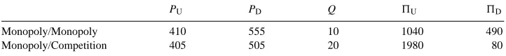
Table 1
Price, quantity, and profit predictionsa
PU PD Q 5U 5D
Monopoly/Monopoly 410 555 10 1040 490
Monopoly/Competition 405 505 20 1980 80
aPrices and profits are in pesos. Profit figures include commissions but are prior to the subtraction of the lump
sum payments of 520 for M/M experiments and 1400 for M/C experiments from the upstream subjects. Although demand is linear, the discreteness causes upstream prices to vary between the two treatments. The actual predicted upstream price with a continuous demand would be 407.5 pesos.
the downstream marginal cost. A linear demand curve was used because it provided the cleanest marginal revenue curve to work with. With a continuous linear demand as well as linear costs, theory predicts that the upstream firm will set the same price regardless of the downstream market structure. In the case of competition downstream, PDwill be equal to downstream marginal cost or PU+100. Substituting PD=PU+100 into Eq. (3) yields Eq. (7), the same PUas in the case of monopoly downstream.3 In all of the experiments, both the upstream and downstream markets had a capacity of 54 units. In the competitive case, three identical firms shared this capacity. The theoretical predictions for upstream and downstream prices, quantities, and profits for these designs can be found in Table 1.
Because the model assumes constant marginal costs, competitive firms earn zero eco-nomic profits in equilibrium. In order to assure that the subjects in the experiments did not earn zero accounting profits, a commission of 4 pesos was paid to each subject whenever
3Graphically, the upstream firm’s marginal revenue curve in the monopoly/competition case is the upstream
he/she sold a unit in both types of experiments. Price offers were restricted to being made in 5 peso increments to avoid a distortion in predictions stemming from this commission. The only effect the commission had was to sharpen the prediction in the monopoly/monopoly case. Because the theory predicts that the upstream firm will squeeze all of the profit out of the downstream on the last unit, the commission provides an incentive to trade the last unit. Since prices could only be made in five peso increments, the upstream firm had no way to extract the four peso commission from the downstream firm on the last unit. This is illustrated in Fig. 1. Marginal revenue equals marginal cost at 10 units for the upstream firm. Upstream price would therefore be set at 410. Marginal cost for the downstream firm would be 410+100 or 510, causing marginal revenue to intersect marginal cost on the step for the 10th unit. Therefore, the downstream firm would be indifferent between selling 9 units and 10 units. The 4 peso commission provides an incentive for the downstream firm to sell this last unit, and the requirement that prices be in 5 peso increments prevents the upstream firm from extracting those 4 pesos from the downstream firm.
An exchange rate of 2.5 pesos/cent was used for the monopolists in each experiment. An exchange rate of 0.25 pesos/cent was used for the competitive firms since the competitive firms were earning only commissions in equilibrium. In the monopoly/monopoly exper-iments, the difference between downstream profits at the Nash prediction and the profits at one unit below the prediction is only the 4 peso commission. The experiments were designed so that a subject’s indifference between choosing the predicted quantity and one unit less would not involve a significant portion of the market. This, along with the linear demand curve, meant that the upstream monopolists in these markets would have earned a great deal of money at the predicted prices. Using a large exchange rate would have flattened out the payoff function more than was felt suitable, so a lump sum payment was taken from the upstream firm each period. Theoretically, this should not affect a subject’s maximizing choices. The lump sum payment was made small enough to allow for a wide variety of choices and mistakes, so final payments to the monopolists still tended to be above average.4
3. Experimental procedures
Thirty-four undergraduates at the University of Arizona participated in these experi-ments. Four monopoly/competition and seven monopoly/monopoly experiments were run. Experiments generally lasted about one and a half hours for both types, and subject pay-ments averaged about $ 16.50 for the monopoly/competitive experipay-ments and $ 28 for the monopoly/monopoly experiments. Each experiment consisted of two practice periods and 15 actual periods, and the subjects were informed of this at the beginning of each experi-ment. The upstream firm was known as the producer, and the downstream firms were known as traders. Final buyers were simulated.
In the monopoly/competition experiments, subjects were brought into the room and told that one of them would have the opportunity to be a single seller, and that we would allow them to earn the right to be that seller. Subjects were given a short trivia quiz, and the high
scorer was awarded the role of producer.5 Each subject was given a set of instructions and record sheets, a buyer demand schedule, and several offer forms. Copies of the instructions for this experiment are available upon request. In this environment, the traders produced to order to avoid any problems associated with carrying inventories or exposing the traders to risk. Each period, the producer was asked to set a price, which the traders were shown immediately. The traders were then invited to submit a contingent price to the buyers. The buyers, who were programmed following the buyer demand schedule, ordered from the traders, given the set of offered prices. The buyers were ordered randomly each period and programmed to approach the low-priced trader first, and in the case of a tie, to randomly choose a trader to deal with. The buyers were programmed this way in order to more closely approximate reality. Because of the competitiveness of these downstream markets, ordering the buyers randomly never reduced the efficiency of the markets. The orders were submitted to the traders, after which the traders made purchase requests from the producer. If the producer did not offer to supply enough units to satisfy the traders, the traders’ purchase requests were processed in a random order which the traders were informed of at the beginning of each period. In each experiment, one subject was paid a fixed payment of $ 15 to run papers back and forth between the subjects and the experimenter to speed processing.
In the monopoly/monopoly experiments, subjects were brought in one pair at a time and randomly assigned the roles of producer and trader. Since subjects were face to face in the monopoly/competition experiments, these experiments were conducted face to face also. An asymmetry of information existed because the producer had enough information to calculate the maximum profit that the trader could earn given each price the producer offered, but the trader had enough information to be able to compute only his own profit. Each period, the producer was asked to post a price which was shown to the trader. The trader then offered a price to the buyers, and knowing the quantity demanded at that price, made his/her purchasing decision.
4. Results
4.1. Comparison of monopoly/monopoly and monopoly/competition outcomes
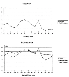
The results from the monopoly/competition experiments are shown in Figs. 2 and 3, and the results from the monopoly/monopoly experiments are shown in Figs. 4–7. The com-petitive downstream price for the monopoly/competition experiments and the downstream best response for the monopoly/monopoly experiments are determined each period from the actual upstream price. Also shown on these graphs are the quantities sold and the market efficiencies6 each period. As a result of the automated buyers and the fact that the subjects
5This practice has become common in experiments in which some portion of the subjects are given an economic
advantage. Hoffman and Spitzer (1985) found that subjects were more likely to fully exploit their economic rights when those rights were earned rather than assigned randomly.
Fig. 7. Monopoly/monopoly results.
always supplied enough units to satisfy the buyers’ demand, these two measures report essentially the same information.
There are several issues to be considered when examining the data. First, do the subjects coordinate their actions in such a way as to achieve the predicted final price and quantity outcomes in the market? Second, do the upstream and downstream subjects behave as the theory predicts? In other words, are final predicted outcomes achieved, and are they achieved through both firms behaving as theory predicts or in some other way? Third, does the change in the downstream market structure affect the efficiency of the markets?
immediately find it unprofitable and return to the competitive price the next period. In the fourth monopoly/competition experiment, although the monopolist had some difficulty in finding the profit-maximizing price, the downstream firms were behaving competitively. No price distortion is present in the downstream market.
In order to examine the questions addressed above more carefully, t-tests on mean prices across experiments were run. All tests are reported using a 5% significance level. In order to determine if the markets behave as theory predicts, the null hypothesis,H0:P¯D=505, is tested against the alternative hypothesis,Ha :P¯D 6=505. Using standard t-tests7 with 11 degrees of freedom, H0cannot be rejected in any of the final five periods.8 In order to examine whether upstream firms behave as theory predicts,H0:P¯U =405 was tested againstHa:P¯U 6=405. Standard t-tests with 3 degrees of freedom indicate that H0cannot be rejected in any of the last five periods. While these tests do not allow us to accept the null hypothesis, they do provide some evidence that the firms are pricing near the theoretical predictions. Further, the mean of the downstream prices across experiments over the last five periods is 505.67, with a standard deviation of 8.76, while the mean of the upstream prices across experiments over the last five periods is 405.50, with a standard deviation of 8.72. Both of these are very close to the predicted values. The vertical structure, as well as each of its component markets, behave in general as theory would predict. This final outcome mirrors the outcome predicted for a vertically integrated firm.
Because these experiments tended to be fairly uninteresting for the subjects and behaved predictably, only four were run. Once price settled down to the competitive price in the downstream market, the traders’ profits were, in effect, determined randomly by the buyer program. From discussions with the downstream subjects following the experiment, it was clear that many of them felt they had little control over the outcome. Three firms provided enough competition in the downstream market to compel the firms to price a marginal cost. Because the downstream firms found that they could do no better than act as price takers, the upstream firm had no incentive to place any restraints on them. Downstream competition effectively controlled their actions. As in the Plott and Uhl middlemen experiments, the middlemen (or traders in this case) took no profit at the expense of the buyers or upstream sellers. Spengler’s assertion that competition in the downstream produces the vertically integrated results and eliminates the incentive for vertical restraints because of the removal of the vertical externality is supported.
In examining the monopoly/monopoly experiments, one can see that there is much more variation in the data than there was in the monopoly/competition data. Subjects seemed to be exploring the profit possibilities. It appeared to be especially difficult for the upstream firm to determine its best strategy as evidenced by the comments of many of the upstream subjects who expressed concern that they could not figure out how the downstream firm was behaving and therefore had difficulty deciding which actions to take.
7Of course t-statistics require the data to be normally distributed, but we have no way of verifying this. However,
nonparametric tests, such as the sign test and the Mann-Whitney test, lead to identical conclusions. Therefore, we will continue to report only the results from the t-tests.
8It should be noted that because of the possible time dependence across periods, these t-tests may not be
The conjecture that these experiments result in the Nash prediction consists of testing the two hypothesesH0: P¯D =555 pesos andH0 :P¯U =410 pesos againstHa :P¯D 6=555 andHa:P¯U6=410, respectively. Using t-tests with 6 degrees of freedom, we cannot reject the hypothesis that the true mean of the final price from the seven monopoly/monopoly experiments is 555 pesos in each of the last five periods.9 However, we can reject in period 14 that the true mean of the upstream prices is 410. The mean of the downstream prices across experiments for the last five periods is 547.43, with a standard deviation of 33.44, while the mean of the upstream prices across experiments for the last five periods is 385.17, with a standard deviation of 34.48. While these averages are not as close to their predicted values as was the case in the monopoly/competition experiments, as discussed before, there is much more variation in the data. Overall we can conclude that there is evidence in these experiments favoring the Nash prediction. However, the rejection of the hypothesis that the true mean of upstream prices is 410 in one of the last five periods may indicate that this is a case where the structure as a whole behaves as theory would predict, but may not be the result of the individual firms behaving as predicted.
In all of the last five periods, we can rejectH0:P¯D=505 pesos in favor ofH0:P¯D> 505 to indicate that the monopoly/monopoly structure tends to result in higher prices than the integrated outcome. This coincides with the results in Fouraker and Siegel, who found support for the Bowley (Nash) rather than the Paretian (integrated) equilibrium in their bilateral bargaining experiments under incomplete information conditions. Subjects here have more information than what was given the Fouraker and Siegel subjects, though it is presented in a different way. Rather than a table of profits, demand is given and subjects can then either compute their own profits or explore the profit options using the market. The upstream firm has enough information to determine the downstream profits if he/she wishes, but it requires some calculations.
An interesting issue to consider in these markets is whether the downstream firms are indeed creating a price distortion, the vertical externality. This can be tested by examining whether the true mean of the actual downstream prices in each period is greater than the mean of what the competitive responses would have been to the upstream prices in each of the last five periods. A t-test for a difference in means with 12 degrees of freedom was performed onH0 :P¯D = ¯PDCRagainstHa : P¯D >P¯DCRwhereP¯DCR is the mean of the competitive responses to the upstream prices in each of the experiments. The only period in which we cannot reject the hypothesis that these two means are the same is in period thirteen. This supports the presence of a vertical externality in these markets.
Spengler’s assertion is that the vertically integrated solution can be duplicated by in-troducing competition in the downstream market, and that both aggregate profit and con-sumer surplus will increase because of this. Using a difference of means test, we can reject the hypothesis in each of the last five periods that aggregate profits in the two structures are equal on average in favor of the hypothesis that aggregate profits are higher in the monopoly/competition markets than in the monopoly/monopoly markets. The null hypoth-esis that consumer surplus is, on average, equal across treatments, can also be rejected in all but one period of the final five periods, in favor of greater consumer surplus in the monopoly/competition treatment. The fact that the null hypothesis could not be rejected in
period 13 is due in large part to experiment MM107, where the firms priced low enough to sell 30 units. Not surprisingly then, using the usual measure of consumer plus producer surplus to measure the efficiency of the markets, in all but one of the last five periods, we can reject the hypothesis that the monopoly/monopoly markets are on average as efficient as the monopoly/competition markets in favor of the hypothesis that the monopoly/competition markets are more efficient. These results strongly support Spengler’s assertion that firms, consumers, and society as a whole are better off with competition, and therefore, a vertically integrated monopolist rather than two successive monopolists.
In addition, we also find that average final prices are higher in the monopoly/monopoly treatments than in the monopoly/competition treatments.H0 : P¯M/M = ¯PM/C could be rejected in favor ofHa :P¯M/M >P¯M/Cin each of the last five periods. The difference in quantities sold between treatments is fairly evident just from examining the data, but we can reject the null hypothesis that the quantities exchanged are equal on average between the two treatments in favor of the alternative hypothesis that the average quantity exchanged in the monopoly/competition experiments is greater than the average quantity exchanged in the monopoly/monopoly experiments in each of the last five periods.
4.2. Examination of individual behavior and coordination
To summarize the results discussed so far, there appears to be strong evidence supporting the Spengler conclusion of a vertical externality when the downstream market is monopo-lized and the argument that the elimination of that externality increases welfare. There are also several questions involving individual behavior and coordination in these experiments which deserve more detailed attention. For example, how close is the downstream firm to its best response function, and does it get better at finding this best response over time? Does the downstream firm’s proximity to its best response function affect how close the upstream firm is to the Nash prediction? How might the upstream firm predict the actions of the downstream firm in order to make its pricing decision? Some models are presented below which are designed to provide some insight into the answers to these questions.
Once the upstream firm has set a price, the downstream firm has a unique best response. The downstream firm’s best response function is a linear function of the upstream price and is specified as follows:10
PDBR =350+0.5PU
In order to determine if downstream prices follow this best response path, a fixed effects model11 was used to estimate
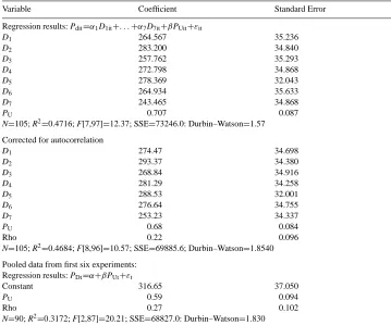
PDit=α1D1it+ · · · +α7D7it+βPUit+εit,
where Dkitequals 1 for experiment k and 0 otherwise. Results from this regression can be found in Table 2. The joint hypothesis thatα1=α2=· · · =α7=350 andβ=0.5 is rejected12
10Because of the discreteness of the demand function, when the upstream price ends in a five, the actual best
response is 2.5 pesos higher than this. The data was adjusted to reflect this.
11A random effects model was rejected which is not surprising with only seven individuals.
Table 2
at the 5% level, which on the surface seems to imply a rejection of the theory. There is some evidence of the presence of serial correlation in the data. However, correcting the data for this still does not prevent H0from being rejected. The results from the corrected regression are also found in Table 2. Closer analysis indicates that rejection of H0stems from MM107, because when tests are conducted on only the first six experiments, we can no longer reject the hypothesis that the intercept is 350 and the slope is 0.5. When only the data from the first six experiments are used, there is no evidence that individual-specific effects are present, so this test can be conducted on pooled data. Results from this regression can also be found in Table 2. This indicates that the downstream firm in MM107 behaved in a significantly different manner than the other downstream monopolists. There does appear to be some evidence that the downstream firms, at least in the first six experiments, are approximating their best response functions.
Another issue that is worth considering is the question of whether the downstream firms are getting better at playing their best strategies over time. This hypothesis was tested by estimating the following equation
Table 3
Regression results: |PDit−PDBRit|=α1D1it+· · · +α7D7it+β1D51it+· · · +β1D57it+εit
Variable Coefficient Standard Error
D1 24.000 4.175
D2 17.000 4.175
D3 15.000 4.175
D4 14.500 4.175
D5 65.000 4.175
D6 4.500 4.175
D7 23.000 4.175
D51 −15.000 7.232
D52 5.000 7.232
D53 −12.000 7.232
D54 3.500 7.232
D55 −40.000 7.232
D56 3.500 7.232
D57 16.000 7.232
N=105; R2=0.6389; F[13,91]=12.39; SSE=15865.0; Durbin–Watson=1.8061
where D5kitis a dummy variable that equals 1 if it is one of the last five periods is experiment k and 0 otherwise.13 Results from this regression can be found in Table 3. The hypothesis that learning is occurring would indicate that theβ’s would be negative.β1,β3, andβ5were all significantly different from zero (β3is only significant at the 10% level while the others are significant at the 5% level) and negative, whileβ2,β4, andβ6were positive and not significantly different from zero.β7was significantly different from 0 and positive, again providing indication that experiment MM107 behaved contrary to the other experiments. It is clear from the graph of MM107 that the downstream price moves away from the best response in the last four periods in that experiment.β6was insignificant because the downstream firm in MM106 was very close to his best response all along and really had very little learning to do. In summary then, we see some limited evidence, except for MM107, that learning may be occurring in this environment in the downstream market.
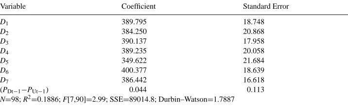
Does the upstream price get closer to the Nash prediction of 410 pesos when the down-stream firms get closer to their best response? In order to answer this question, the fixed effects model below was estimated:
|PUit−410| =α1D1it+ · · · +α7D7it+β|PDit−1−PDBRit−1| +εit.
Coefficient estimates and standard errors from this regression can be found in Table 4. Upstream prices getting closer to the Nash prediction as downstream firms get better at finding their best responses would imply aβ>0. The hypothesis thatβ=0 cannot be rejected in this model.14 This model provides no evidence that the closeness of downstream price to its best response is significant in determining how close the upstream price is to the Nash prediction.
Table 4
The downstream firm has a clear best response in these markets. The upstream firm, however, must predict what the downstream firm’s response will be in order to choose a ‘best response’. Three models of this predictive process are hypothesized. A myopic
prediction occurs when the upstream firm assumes that the downstream firm will post the
same price this period as it did last period. The best response to this prediction is for the upstream firm to post
PUt =α+βPFt−1 where α= −100 and β=1 (a) A constant markup prediction occurs when the upstream firm predicts that the down-stream firm will mark the price up this period by the same amount as it did the last period. The best response to this prediction is to post
PUt =α+β(PDt−1−PUt−1) where α=455 and β= −0.5. (b) An OLS prediction assumes the upstream firm observes the downstream firm’s pricing responses and estimates a linear function relating that price to the upstream price he/she posted. This estimate is updated after each period. This prediction involves the upstream firm running the regression PDt=γ+δPUt+εteach period with all the observations available up to that point in time. Once he has made an estimate of a and b, his best response is to charge
Two separate fixed effects models were run to estimate models (a) and (b).15 Results from both models can be found in Tables 5 and 6. In both cases, the hypotheses that the coefficients are equal to their theoretical values are rejected. In addition, the R2’s for both models are very low. These are joint tests of the prediction model and whether the upstream firms respond optimally to their predictions. If the upstream firms are making
15This method was not applied to model (c) because model (c) would require estimatingγ andδin stage 1
Table 5
either myopic or constant markup predictions of downstream behavior, there is no evi-dence that they are using the best responses to these predictions to make their pricing decisions.
In order to discover if there is any evidence that the upstream firm is using an OLS-type prediction to choose his price, a test of the equality of means between the actual up-stream prices and the best response prices given OLS predictions was conducted. We cannot reject the hypothesis that the true means of the two populations are equal in any of the last eight periods, suggesting some evidence that the upstream firms are pricing on average as if they are making optimal responses to an OLS prediction of downstream behavior.
5. Conclusion
The experiments reported here provide support for Spengler’s double marginalization theory. The vertical externality is present in laboratory markets when vertical markets are controlled by monopolists, providing evidence that a chain of monopolies is less efficient than a single monopolist. Prices in the monopoly/competition markets approached the in-tegrated solution, and prices in the monopoly/monopoly markets supported the double marginalization prices. The profit incentive for an upstream firm to control downstream decisions in the monopoly/monopoly experiments was present. Many of the upstream sub-jects said that they felt like they didn’t have much control, and that it was the downstream firm that decided how much profit they were going to make. This is further evidence that the vertical externality provides the upstream firm with an incentive to control the actions of the downstream firm. The vertical externality is removed when the downstream market is characterized by competition and welfare is increased. The incentive for the use of ver-tical restraints or integration is not present in this simple environment once competition is introduced.
The experimental examination of vertical issues has many possible directions for future research. The experiments reported in this paper indicate that in the basic vertical structure, there may be an incentive to use vertical restraints or to integrate when the downstream market is not competitive. The experimental design could be modified to examine other issues of interest. For instance, how important are the information conditions? What hap-pens when downstream firms no longer produce to order? What if a variable proportions production function were introduced in the downstream market? These questions remain open to further examination.
Acknowledgements
The financial support of the Economic Science Laboratory at the University of Arizona, Tucson, Arizona 85721 is gratefully acknowledged.
References
Fouraker, L.E., Siegel, S., 1963. Bargaining Behavior, McGraw-Hill, New York.
Goodfellow, J., Plott, C.R., 1990. An experimental examination of the simultaneous determination of input prices and output prices. Southern Economic Journal 56, 969–983.
Harrison, G.W., McKee, M., 1985. Monopoly behavior, decentralized regulation, and contestable markets: an experimental evaluation. Rand Journal of Economics 16, 51–69.
Harrison, G.W., McKee, M., Rutström, E.E., 1989. Experimental evaluation of institutions of monolopy restraint (Chapter 3). In: Green, L., Kagel, J. (Eds.), Advances in Behavioral Economics, Vol. 2. Albex Press, Norwood, N.J., pp. 54–94.
Hoffman, E., Plott, C.R., 1981. The effect of intertemporal speculation on outcomes in seller posted offer auction markets. Quarterly Journal of Economics 96, 223–241.
Hoffman, E., Spitzer, M.L., 1985. Entitlements, rights, and fairness: An experimental examination of subjects’ concepts of distributive justice. Journal of Legal Studies 14, 259–297.
Plott, C.R., Uhl, J.T., 1981. Competitive equilibrium with middlemen: an empirical study. Southern Economic Journal 47, 1063–1071.
Smith, V.L., 1981. An empirical study of decentralized institutions of monopoly restraint. In: Horwich, G., Quirk, J. (Eds.), Essays in Contemporary Fields of Economics in Honor of E.T. Weiler, (1914–1979). Purdue University Press, West Lafayette, pp. 83–106.
Spengler, J., 1950. Vertical integration and anti-trust policy. Journal of Political Economy 347–352. Tirole, J., 1988. The Theory of Industrial Organization. The MIT Press, Cambridge, Mass.
Williams, A.W., 1979. Intertemporal competitive equilibrium: on further experimental results. In: Vernon, L. Smith, (Ed.), Research in Experimental Economics, Vol 1. JAI, Greenwich, Conn.