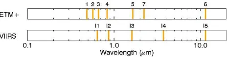
Figure 1. A comparison of the central wavelengths of the Landsat 7 ETM+ bands and the VIIRS I-Bands.
A RAPID CLOUD MASK ALGORITHM FOR SUOMI NPP VIIRS IMAGERY EDRS
M. Piper a,*, T. Bahr b a
INSTAAR / CSDMS, University of Colorado Boulder, U.S.A. – [email protected] b
Exelis VIS GmbH, 82205 Gilching, Germany – [email protected]
KEY WORDS: Suomi NPP, VIIRS, Cloud Mask Algorithm, Classification, Skill Scores
ABSTRACT:
Suomi National Polar-orbiting Partnership (NPP) is the first of a new generation of NASA's Earth-observing research satellites. The Suomi NPP Visible Infrared Imaging Radiometer Suite (VIIRS) collects visible and infrared views of Earth's dynamic surface processes. This NPP mission produces a series of Environmental Data Records (EDRs). As accurate information on cloud occurrence is of utmost importance for a wide range of remote-sensing applications and analyses, we developed a cloud mask algorithm, adapted from the Landsat 7 Automatic Cloud Cover Assessment, for use with the VIIRS Imagery EDRs. The algorithm consists of a sequence of pixel-based tests that use thresholds on VIIRS top-of-atmosphere reflectances and brightness temperatures. Our cloud mask algorithm provides a simpler, though less informative and robust, alternative to the VIIRS Cloud Mask (VCM) Intermediate Product, with the advantage in that it can be applied to a higher spatial resolution VIIRS Imagery EDR. The algorithm is compared with the VCM in three case studies.
*
Corresponding author
1. INTRODUCTION
Suomi National Polar-orbiting Partnership (NPP) is the first of a new generation of NASA's Earth-observing research satellites that observes many facets of our changing Earth. Since 2011 it collects and distributes remotely-sensed land, ocean, and atmospheric data to the meteorological and global climate change communities. The Suomi NPP Visible Infrared Imaging Radiometer Suite (VIIRS) has a 22-band radiometer similar to the MODIS instrument. It collects visible and infrared views of Earth's dynamic surface processes, such as wildfires, land changes, and ice movement. VIIRS also measures atmospheric and oceanic properties, including clouds and sea surface temperature. This NPP mission produces a series of Environmental Data Records (EDRs).
As accurate quality information on cloud occurrence is of utmost importance for a wide range of remote-sensing applications and analyses, we developed a new cloud mask algorithm, based on the Landsat 7 automatic cloud cover assessment (Irish, 2000; Irish et al., 2006), for use with the VIIRS Imagery EDRs. Though the cloud mask algorithm produces results that are less accurate than the VIIRS Cloud Mask (VCM) Intermediate Product (JPSS, 2015), it has an advantage in that it can be quickly calculated from a VIIRS Imagery EDR and used to assess cloud cover at the EDR's 375 m nadir resolution.
2. CLOUD MASK ALGORITHM
The cloud mask algorithm exploits the similarity between the multispectral bands of Landsat-7 ETM+ and NPP VIIRS Imagery, as shown in Figure 1.
The cloud mask algorithm (hereafter VIBCM, for VIIRS I-Band Cloud Mask) consists of a sequence of six pixel-based tests that use thresholds on VIIRS top-of-atmosphere reflectances,
brightness temperatures, and combinations of these measurements. Each test returns a binary (pixel is clear or cloudy) result. For a pixel to be classified as cloudy, it must pass all six tests:
1. Brightness threshold. Pixels in I1 with a reflectance greater than 0.08 are classified as cloudy.
2. Normalized difference snow index. Pixels with a Normalized Difference Snow Index (NDSI) greater than 0.7 and I2 reflectance greater than 0.11 are classified as cloudy. With VIIRS, NDSI is calculated as (I1 - I3) / (I1 + I3) (JPSS, 2011).
3. Temperature threshold. Pixels in I5, the thermal band, with brightness temperatures less than 312 K are classified as cloudy. This threshold value is higher than the value of 300 K used in Irish (2000) because warm clouds were being excluded.
4. Band I3-I5 composite. In the composite defined by (max(I3) - I3)*I5, pixels less than a threshold of 410 K, determined by sensitivity analysis, are classified as cloudy. In Irish (2000), a threshold of 225 K was chosen by a similar analysis.
6. Band I2/I3 ratio. Useful for identifying rocky or sandy areas, pixels in this test with ratios greater than 1.0 are classified as cloudy.
Unless otherwise noted, threshold values in the tests are taken from Irish (2000). Filters 6 and 8 from Irish (2000) use Landsat 7 ETM+ bands that don’t match the VIIRS Imagery bands, and so are omitted in the VIBCM. Irish also identifies ambiguously cloudy pixels, then uses a second pass over the data to help classify these pixels. This second pass is not employed in the VIBCM.
3. EXPERIMENT
The VIBCM was tested against the VCM on three daytime, ascending, VIIRS scenes, listed in Table 1.
Location Acquisition
Start Time Orbit Description
Scene 1 Hawaii
2015-Feb-06 23:18:58.504
16991 This scene is dominated by warm ocean and warm
5322 Cold clouds from two weather systems
Table 1. The VIIRS scenes used to compare the VIBCM to the VCM.
In each scene, the VCM, at 750 m resolution, was registered to the VIBCM and interpolated to the VIIRS Imagery resolution of 375 m using nearest-neighbor sampling. We chose to use UTM, with the WGS-84 datum, as the common projection for the masks. We chose to count VCM pixels that are probably or confidently cloudy, with medium to high mask quality, as cloudy for the comparison.
To quantify the relationship between the VCM and the VIBCM, we constructed a 2 x 2 contingency table (Stanski et al., 1989) for each of the three scenes, with the VCM representing the "observed" variable and the VIBCM the "forecast" variable. As shown in Table 2, each pixel has a binary classification –cloudy or not cloudy – for each algorithm. With the VCM as
the basis for comparison, there are two cases where the VIBCM gives the correct result: a "hit" (cell (a) in Table 2), when a pixel is classified as cloudy by both algorithms, and a "correct Table 2. A contingency table for the frequency of cloudy pixels
in the VCM and the VIBCM.
Skill scores can be derived from the contingency table values (Stanski et al., 1989). The skill scores used in this experiment are listed in Table 3 and described below.
Name Formula
Table 3. Skill scores derived from the contingency table in Table 2.
1. Bias compares the frequency of forecasts to the frequency of actual occurrences. Bias ranges from zero to infinity, with an unbiased score of one. Here, a bias less than one indicates fewer cloudy pixels are present in the VIBCM than in the VCM.
2. Hit rate measures the proportion of observed events that were correctly forecast. The range of the hit rate is zero to a perfect score of one.
3. Accuracy is the ratio of correct events (both cloud and no cloud) to the total number of events. It ranges from zero to a perfect score of one.
5. Critical Success Index accounts for false alarms and misses after removing correct negatives. It ranges from zero to a perfect score of one.
6. Heidke Skill Score measures the fraction of correct forecasts after removing those due to chance. This score ranges from minus infinity to a perfect score of one, with a score of zero equal to chance, and negative scores indicating skill less than chance.
7. Hanssen-Kuiper Skill Score separates the forecasted "Yes" cases from "No" cases. It ranges from minus one to one, with a perfect score of one, and chance equal to zero. All code used in creating the VIBCM and in comparing it with the VCM are open source and freely available from Piper (2015), under the MIT License.
4. RESULTS AND DISCUSSION
To provide a qualitative comparison of the cloud masks, the three VIIRS scenes are previewed in Figures 2, 3, and 4.
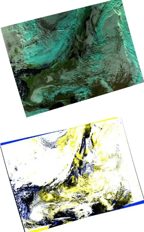
In the first position of each Figure, an I3-I2-I1 false-color composite image, with a two percent linear stretch applied, is displayed to give a visual depiction of the cloud cover in the scene. In the second position, the VIBCM and VCM computed for a scene are added graphically as binary images. In the result, a white pixel is identified as cloudy by both masks, a black pixel is not a cloud in either mask, a blue pixel is a cloud only in the VCM, and a yellow pixel is a cloud only in the VIBCM. The white, black, blue, and yellow colors in these images provide a visual representation of the contingency table computed for each scene. The areas around the edges of these images, where the registered scenes do not overlap, are excluded from further calculations.
Tables 4, 5, and 6 give quantitative comparisons of the cloud mask algorithms for each scene of the study. Each Table displays pixel counts, cloud fractions, a contingency table, and the derived statistics described in Table 3.
Total pixels
Cloudy pixels Cloud fraction
VCM VIBCM VCM VIBCM
49390823 28434565 21255906 0. 5757 0.4304
Cloud in VCM
Yes No (totals)
Cloud in Yes 20474434 781472 21255906 VIBCM No 7960131 20174786 28134917 (totals) 28434565 20956258 49390823
Bias Hit rate Accuracy FA rate CSI HSS KSS
0.7475 0.7201 0.8230 0.0373 0.7008 0.6533 0.6828
Table 4. Cloud fraction, contingency tables, and skill scores for Scene 1 (Hawaii).
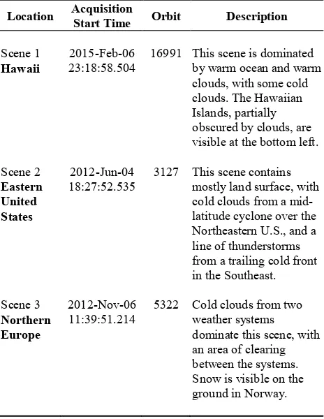
Scene 1, which includes Hawaii in the lower left, is roughly split between cloudy and clear skies. In this scene, the VCM and the VIBCM largely agree on the locations of the cloudy and clear areas. This is supported qualitatively by the predominance of white and black pixels, respectively, in the lower panel of Figure 2. Quantitatively, Table 4 shows that this agreement on cloudy and clear pixels is born out by a high accuracy value. Table 4 also shows that the VIBCM compares favorably with the VCM by other measures; for example, CSI is much greater than zero, indicating a high number of correct events relative to false alarms and misses, and the false alarm rate is close to zero.
However, there are a significant number of misses by the VIBCM, as visually indicated by the blue pixels in the bottom panel of Figure 2. These misses cause a disparity in the computed cloud fraction, pull down skill scores like the hit rate, HSS, and KSS, and give a bias less than one because of the higher number of cloudy pixels identified by the VCM. Figure 2 shows that the misses tend to be concentrated around the edges of the cloudy regions. One explanation may be that the VIBCM does a poorer job of identifying clouds that aren’t optically Figure 2. VIIRS I3-I2-I1 false color composite (above)
thick. Another is that the conditions we used to define a cloud in the VCM (i.e., a pixel marked as probably or confidently cloudy, with medium to high quality) may be too loose. When we increased the Filter 4 threshold value to 440 K in this scene, the number of misses decreased by 46 percent, to 4303254, with concomitant increases in hit rate, accuracy, HSS and KSS skill scores. This hints at a nonlinear temperature dependency in this filter.
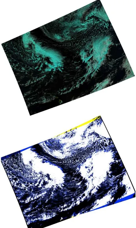
In Scene 2, covering the Eastern United States and Canada, about half of the area is cloud-covered, with a mid-latitude cyclone exiting to the northeast, and a line of scattered thunderstorms along a trailing cold front to the south, as shown in the top panel of Figure 3.
As in Scene 1, there is good qualitative agreement between the cloud masks, as evidenced by the prevalence of white (cloudy) and black (clear) pixels in the bottom panel of Figure 3. The Figure also shows that the VIBCM is still missing clouds picked up by the VCM. The blue pixels indicative of these misses again tend to be found around the edges of deeper cloud banks. Although this occurs throughout the scene, it is especially noticeable in the southern portion.
However, the VIBCM may not be entirely at fault for these misses: in the bottom panel of Figure 3, we noticed that the VCM is picking up the Mississippi and Missouri rivers. There is also an area of stratiform clouds over Lake Huron that, by inspection of the top panel of Figure 3, does not appear to cover as wide an area as indicated by the VCM. This strengthens that argument that we may not have been sufficiently careful in setting conditions for cloudy pixels in the VCM.
One difference between the current scene and Scene 1 is the doubling of the number of yellow false alarm pixels, where the VIBCM identifies a pixel as cloudy, while the VCM does not. Figure 3 shows that the false alarm pixels are grouped in the northeast corner of the scene. The location of the false alarm pixels again suggests an unattributed temperature dependency in the VIBCM.
Total pixels
Cloudy pixels Cloud fraction
VCM VIBCM VCM VIBCM
49327866 30521583 25345629 0.6187 0.5138
Cloud in VCM
Yes No (totals)
Cloud in Yes 23764738 1580891 25345629 VIBCM No 6756845 17225392 23982237 (totals) 30521583 18806283 49327866
Bias Hit rate Accuracy FA rate CSI HSS KSS
0.8304 0.7786 0.8310 0.0841 0.7403 0.6597 0.6946
Table 5. Cloud fraction, contingency tables, and skill scores for Scene 2 (Eastern United States).
Table 5 shows that, for this scene, like Scene 1, the total number of cloudy pixels, as well as the cloud fraction, are higher in the VCM. This is due to the number of misses (blue) by the VIBCM. However, the current scene actually has fewer misses than Scene 1, which gives a higher hit rate.
As in Scene 1, the accuracy in this scene is high. The count of correct cloudy pixels (white) and correct clear areas (black) are each an order of magnitude larger than the miss and false alarm (yellow) values. Likewise, the CSI score remains high because the number of correct cloudy pixels far outnumber misses and false alarms.
The bias score is in favor of the VCM, again because of the misses in the VIBCM. The bias is less than that in Scene 1, though, because of higher number of false alarm pixels in the current scene. The false alarm rate is higher than in Scene 1, but it is still close to zero.
The HSS and KSS scores for this scene are high, and are similar to those in Scene 1. Both are closer to one (a perfect prediction) than zero (random chance).
Figure 3. VIIRS I3-I2-I1 false color composite (above) and cloud mask comparison (below) images for Scene 2
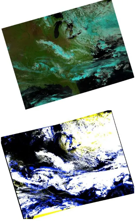
Two storm systems dominate the weather over Northern Europe in Scene 3, with snow on the ground in Norway, in the northern half of Sweden, and in the Alps (NCDC, 2015). Clouds (white pixels) prevail in this scene.
Note that, in the bottom panel of Figure 4, there are far fewer blue pixels, denoting misses by the VIBCM, than in the previous two scenes. There are, however, more yellow pixels, indicating false alarms by the VIBCM. The VIBCM misclassifies the snow on the ground in Norway and Sweden as cloud. On the other hand, the VIBCM appears to correctly identify two low cloud banks to the southwest of Stockholm, and one to the north of Berlin, none of which are picked up by the VCM.
Table 6 shows that the number of false alarm pixels (yellow) is approximately three times as high as Scene 2. However, the number of misses (blue) is nearly three times lower. The false alarm rate is five times as high as in Scene 2. Note that this is due, in part, to the clouds missed by the VCM described above, so this number may be inflated.
Overall, the VIBCM compares well with the VCM in this scene, with the highest hit rate, accuracy and CSI scores of the three
scenes, and the lowest bias. These high scores are the result of the large number of cloudy pixels classified by both masks.
Total pixels
Cloudy pixels Cloud fraction
VCM VIBCM VCM VIBCM
49436935 36149374 39745887 0.7312 0.8040
Cloud in VCM
Yes No (totals)
Cloud in Yes 34155952 5589935 39745887 VIBCM No 1993422 7697626 9691048 (totals) 36149374 13287561 49436935
Bias Hit rate Accuracy FA rate CSI HSS KSS
1.0995 0.9449 0.8466 0.4207 0.8183 0.5732 0.5242
Table 6. Cloud fraction, contingency tables, and skill scores for Scene 3 (Northern Europe).
When we lowered the Filter 4 threshold to 390 K, it resulted in a decrease of 23 percent in the number of false alarm pixels, to 4280523. This, in turn, decreased in the false alarm rate and the bias. Accuracy, along with HSS and KSS, increased. CSI remained approximately the same.
5. CONCLUSIONS
We developed a cloud mask algorithm (the VIIRS I-Band Cloud Mask, or VIBCM) based on the Landsat 7 ETM+ Automatic Cloud Cover Assessment. To assess its ability to identify clouds, we compared it, both qualitatively and quantitatively, with a cloud mask derived from the VIIRS Cloud Mask (VCM) Intermediate Product using a case study of three VIIRS scenes that varied in location and season. The results indicate, by various skill scores, a quantitatively good match between the two cloud masks; for example, the accuracy, defined as the sum of cloudy and clear pixels classified by both masks, divided by the total number of pixels in a scene, is above 80 percent in each of the scenes. However, there remains room for improvement.
The VIBCM provides the following advantages:
It can quickly be computed from the five bands of a VIIRS Imagery EDR. No outside sources are needed.
It computes a mask at the Imagery EDR resolution of 375 m nadir instead of the SDR resolution of 750 m. The VIBCM also has disadvantages:
It is not as accurate as the VCM: cloudy pixels are frequently missed or misidentified.
It is not as detailed as the VCM: there are no confidence flags for cloudy pixels, and no distinction between high clouds, low clouds, fog, smoke, and shadow (JPSS, 2015). Figure 4. VIIRS I3-I2-I1 false color composite (above)
There are three unresolved issues in the VIBCM that merit future work. The first is an investigation of what appears to be a temperature dependency in the threshold value of Filter 4. As the I5 brightness temperatures decreased from Scene 1 (Hawaii, warm) through Scene 3 (Europe, cold), the number of misses by the VIBCM decreased, and the number of false alarms increased. When we experimented with different threshold values in each scene, some of misses and false alarms were converted into hits. It would be better to perform an extended case study, where the use of many scenes might help quantify an empirical relationship between the threshold temperature in Filter 4 and its response. Alternately, the two-pass technique used by Irish (2000), which we chose not to implement in the VIBCM, could help address this issue. The second unresolved issue lies in what we have chosen to define as a cloud in the VCM; that is, any pixel that is probably or confidently cloudy, with medium to high mask quality. As described above, this definition produces false alarms in Scene 2, and misses in Scene 3. We want to be careful in stating that we do not fault the VCM for this issue; rather, we may need to be more careful in our use of the quality flags produced by the VCM. In future work, we will explore how seasonal and latitudinal conditions on how the VCM is used affect the comparison with the VIBCM.
The third issue that merits further study is differentiating between clouds and snow. Only one scene in our case study had snow, and the VIBCM failed to identify it. Improving this behavior will require additional work with a range of VIIRS scenes that contain snow, cold surface temperatures, and cold clouds.
ACKNOWLEDGMENTS
MP gratefully acknowledges the help of Curtis Seaman (CIRA/Colorado State University) in dealing with bowtie deletion issues in the VIIRS imagery.
REFERENCES
Irish, R.R., 2000. Landsat 7 automatic cloud cover assessment. Proceedings of SPIE, 4049, pp. 348–355.
Irish, R.R., Barker, J.L., Goward, S.N., Arvidson, T., 2006. Characterization of the Landsat-7 ETM+ Automated Cloud-Cover Assessment (ACCA) algorithm. Photogrammetric Engineering & Remote Sensing, 72 (10), pp. 1179–1188. Joint Polar Satellite System (JPSS), 2015. Joint Polar Satellite System (JPSS) Operational Algorithm Description (OAD) Document for VIIRS Cloud Mask (VCM) Intermediate Product (IP) Software. http://npp.gsfc.nasa.gov/sciencedocuments/2015-03/474-00062_OAD-VIIRS-Cloud-Mask-IP_H.pdf.
(10.03.2015)
Joint Polar Satellite System (JPSS), 2011. Joint Polar Satellite System (JPSS) VIIRS Snow Cover Algorithm Theoretical Basis Document (ATBD). http://npp.gsfc.nasa.gov/sciencedocuments/ ATBD_122011/474-00038_VIIRS_Snow_Cover_ATBD_Rev-_20110422.pdf. (10.03.2015)
National Climatic Data Center (NCDC), 2015. Europe/Asia Snow Cover. http://www.ncdc.noaa.gov/snow-and-ice/snow-cover/ea/20121105-20121107. (23.03.2015)