ANNUAL FOREST MONITORING AS PART OF THE INDONESIA’S NATIONAL
CARBON ACCOUNTING SYSTEM
Kustiyo a, *, O. Roswintiarti a, A. Tjahjaningsiha,R. Dewantia, S. Furbyb, J. Wallaceb a
Indonesian National Institute of Aeronautics and Space (LAPAN), Deputy for Remote Sensing Affairs, Indonesia – [email protected]
b
CSIRO, Digital Productivity Flagship, Perth, Australia – [email protected]
THEME: BIOD / Biodiversity. Special session: "Trends in operational land cover mapping"
KEY WORDS: Multi-temporal, Landsat, Land Cover, Monitoring, Forestry, Change Detection
ABSTRACT:
Land use and forest change, in particular deforestation, have contributed the largest proportion of Indonesia’s estimated greenhouse gas emissions. Indonesia’s remaining forests store globally significant carbon stocks, as well as biodiversity values. In 2010, the Government of Indonesia entered into a REDD+ partnership. A spatially detailed monitoring and reporting system for forest change which is national and operating in Indonesia is required for participation in such programs, as well as for national policy reasons including Monitoring, Reporting, and Verification (MRV), carbon accounting, and land-use and policy information.
Indonesia’s National Carbon Accounting System (INCAS) has been designed to meet national and international policy requirements. The INCAS remote sensing program is producing spatially-detailed annual wall-to-wall monitoring of forest cover changes from time-series Landsat imagery for the whole of Indonesia from 2000 to the present day. Work on the program commenced in 2009, under the Indonesia-Australia Forest Carbon Partnership. A principal objective was to build an operational system in Indonesia through transfer of knowledge and experience, from Australia’s National Carbon Accounting System, and adaptation of this experience to Indonesia’s requirements and conditions. A semi-automated system of image pre-processing (ortho-rectification, calibration, cloud masking and mosaicing) and forest extent and change mapping (supervised classification of a ‘base’ year, semi-automated single-year classifications and classification within a multi-temporal probabilistic framework) was developed for Landsat 5 TM and Landsat 7 ETM+. Particular attention is paid to the accuracy of each step in the processing. With the advent of Landsat 8 data and parallel development of processing capability, capacity and international collaboration s within the LAPAN Data Centre this processing is being increasingly automated. Research is continuing into improved processing methodology and integration of information from other data sources.
This paper presents technical elements of the INCAS remote sensing program and some results of the 2000 – 2012 mapping.
* Corresponding author. This is useful to know for communication with the appropriate person in cases with more than one author.
1. INTRODUCTION
1.1 Background
Land use and forest change, in particular deforestation, have contributed the largest proportion of Indonesia’s estimated green house gas (GHG) emissions. Indonesia’s remaining forests store globally significant carbon stocks, as well as biodiversity values. In 2010, the Government of Indonesia entered into a REDD+ (Reducing Emissions from Deforestation and Forest Degradation and the role of conservation, sustainable management and enhancement of forest carbon stocks) partnership. President Yudhoyono pledged to reduce Indonesia’s GHG emissions by up to 26% below business as usual levels in 2020, with consideration of increasing this to 41% with sufficient international support. A spatially detailed monitoring and reporting system for forest change which is national and operating in Indonesia is required for participation in such programs, as well as for national policy reasons including Monitoring, Reporting, and Verification (MRV), carbon accounting, and land-use and policy information.
The monitoring system was designed in response to existing and anticipated international agreements and frameworks, including developments from the Kyoto protocol, IPCC guidelines and expectations for REDD+. The design requirements included (a) national coverage (b) sub-hectare spatial resolution (c) capacity to monitor historic changes over at least ten years, and to continue monitoring into the future. Landsat imagery, on account of its resolution and historic archive, was the only feasible data source to meet these requirements.
Figure 2. Locations and numbers of high resolution imagery (closed red squares) for Sulawesi shown on 2008 Landsat TM mosaics (bands 3, 4, 5 in BGR).
source for coming years, and SPOT-5/6/7 can be used for improving the accuracy of the products.
A detailed explanation of the forest monitoring system is provided in LAPAN (2014). The technical description that follows is a summary extracted from this methodology document.
1.2 Indonesia’s National Carbon Accounting System
Indonesia's National Carbon Accounting System (INCAS) was a program that has been designed to build a credible and sustainable system in Indonesia to account for green house gas (GHG) and allow for robust emissions reporting from Indonesia’s land sector, with full national coverage. It was undertaken in response to national and international policy drivers with a focus on forests and forest change.
The program consists of two major technical components; the remote sensing component, and the emissions estimation component. The remote sensing component, Land Cover Change Analysis (LCCA), provides spatially detailed monitoring for the whole country of annual forest changes using satellite remote sensing imagery. The emissions estimation component includes forest biomass measurement, forest disturbance mapping, and carbon stock assessment and emissions estimations to produce GHG accounts.
The INCAS remote sensing program commenced in 2009, under the Indonesia-Australia Forest Carbon Partnership (IAFCP). A principal objective was to build an operational system in Indonesia through transfer of knowledge and experience, from Australia’s National Carbon Accounting System, and adaptation of this experience to Indonesia’s requirements and conditions.
1.3. Objective
The initial objective of the forest monitoring as part of INCAS was to map the annual extent of forested land and the annual changes using time-series Landsat imagery for the whole of Indonesia for the 12-year period of 2000 - 2012.
For this objective, forest cover is defined as physical land cover irrespective of tenure; as a collection of trees with height greater than 5 metres and having greater than 30% canopy cover. Plantations of oil palm and coconut palm are considered as non-forest. All other land cover is considered non-forest.
2. SOURCES OF DATA AND INFORMATION
2.1 Landsat imagery
Landsat imagery was chosen as the only feasible data source to provide annual forest monitoring. Landsat-5 is the preferred source for most of the period due to a technical problem with the scan line corrector (‘SLC-off’) which affected Landsat-7 from mid-2003. However in cases where cloud cover affects available Landsat-5 imagery, Landsat-7 imagery may be more useful.
The most complete archive of Landsat-5 imagery for western Indonesia for the period of 2000-2012 was held at Thailand’s
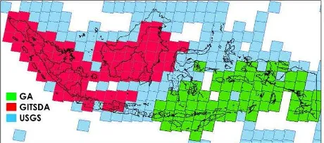
GISTDA receiving station; Australia’s archive, held at Geoscience Australia (GA) covers far eastern Indonesia (Papua to eastern Nusa Tenggara) with Landsat-5 and Landsat-7 imagery. LAPAN’s receiving station at Parepare covers all of Indonesia, except for the very western tip of Sumatra, but only limited scenes had been archived. The main source of data for the central region was thus the USGS archive, which was far from complete for Landsat-5 as it consists of a sample of scenes selected for on-board storage and downloaded in the US. GA coordinated the image acquisition of Landsat imagery from these international data agencies.
Figure 1. Indicative extent of spatial coverage of the GISTDA, GA and USGS Landsat archives.
2.2 High resolution imagery
Samples of high resolution satellite imagery were acquired for supporting forest monitoring. These were used for purposes of accurate interpretation of land cover in the forest mapping for supervised classification and forest review stages of the program. These tasks required an image resolution which could provide estimates of tree density, and indications of height from shadow. A resolution of two metres or better is required for these purposes.
The high resolution images were selected to contain cloud-free samples of all important cover types. It is important that the images contain multiple cover types and/or a mixture of tree density so that boundaries between land cover classes can be interpreted. Figure 2 shows the high-resolution image locations for Sulawesi regions. In total, 271 high resolution images were purchased by IAFCP for Kalimantan, Sumatra, Papua and Sulawesi regions, other high resolution images were purchased by LAPAN and the Ministry of Agriculture for Java region, and for other regions, the images available in Google Earth(TM) were used.
2.3 Expert knowledge and map data
combination with the high resolution imagery, and the available maps, this human expertise with regional knowledge provided essential guidance to the production and assessment of the forest extent base maps
3. METHODOLOGY
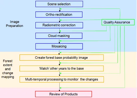
There are a number of steps to produce the annual forest extent and change maps; the outputs from each step typically are required inputs for the subsequent step. The progression of processing steps is shown in the flowchart in Figure 3.
Figure 3. Flowchart of the steps in the annual forest monitoring processing sequence.
The steps in blue form, showed in Figure 3, are the data preparation processing performed on individual images. The steps in orange form are the forest extent and change mapping processing performed on the image mosaics. The final step is a review of the products.
After each step in the processing there is a quality assurance (QA) process to check that the method has been correctly applied and that the results meet required accuracy standards. If an image does not meet the standards for that step, the cause is investigated and the image will be reprocessed to correct the problem and checked again. The next step is not commenced until the current step is successfully completed.
3.1 Image Preparation
First the images to be used in the annual forest monitoring are selected. The selected images must be aligned geographically to each other and to other map data. Corrections to make the image values more consistent through time are then made. Contaminating data – such as cloud and shadow, haze, smoke and image noise - that obscure the ground cover are then masked from the images. The individual images are then mosaiced into larger units – mosaic tiles – to streamline the subsequent processing. Together these steps form the data preparation stage of the processing.
3.1.1 Scene selection: To map annual forest extent and change, one cloud-free view of the land cover each calendar year was required. A single clear image is ideal and sufficient, but due to cloud cover this is a rare occurrence in tropical regions like Indonesia. The aim of the scene selection is to provide annual coverages of Indonesia with maximum
cloud-free land area using the minimum number of scenes. The selection criteria were designed to provide best inputs to the subsequent forest extent mapping process.
3.1.2 Ortho-rectification: Accurate scene registration within and between years is essential for a monitoring program so that misregistration errors are not confused with land cover change (Townshend et al. 1992). As the equator passes through Indonesia a decision needed to be made about the projection for the individual images. For convenience and consistency all images are referenced to NUTM coordinates (WGS84 datum). All images are resampled to 25m pixel size for simple alignment with metric map scales and area calculations.
The ortho-rectification processing needs a rectification image base. The Global Land Survey 2000 (GLS2000) data (USGS 2009, http://glcf.umd.edu/data/gls/) was selected as rectification image base for the whole of Indonesia. The GLS2000 is formed from Landsat 7 ETM+ images and is a reprocessed version of the Global Land Cover Facility (GLCF) 2000 GeoCover(TM) collection (Tucker et al 2004) using Shuttle Radar Topography Mission (SRTM) digital topography and improved geodetic control (Gutman et al. 2008). The data is provided in GeoTIFF format with a UTM projection using the WGS-84 datum at 30m pixel resolution.
All Landsat images must be ortho-rectified and registered to the geometric base to produce individually rectified images, which will eventually result in a consistently-registered time series of imagery for all of Indonesia. The preferred processing level for historic imagery was path-oriented (nominal orientation) to enable full ortho-rectification correction.
To register a new image to the base, correlation matching is used to locate predefined physical features from the ortho-rectified base image in the new image. The coordinates of the center of these features are then used as the GCPs to formulate the transformation between the new image and the base.
A library of these predefined feature locations was created for every path/row for Indonesia. These locations are called ‘Master GCPs’. They are also referred to as ‘GCP chips’ in some applications. Two sets of Master GCPs were selected. One – the Master Registration GCPs – serve to generate ground control points for fitting the ortho-rectification model. The other – the Master Check GCPs – serve as sets of independent check points that are used during the quality assurance stage to assess how well the processed image is registered to the base.
Ortho-rectification correction fits a sequence of three models in the actual ortho-rectification process of the raw image. The details are found in Wu (2008). This approach achieves accurate ortho-rectification without the requirement for sensor and orbital ephemeris information, only an approximate satellite height. The approach has been compared to established implementations using satellite orbital modelling and results agree very closely. The resampling kernel used is 16-point sinc with Kaiser windowing.
viewing angles. In order to apply subsequent numerical classification processing, it is desirable that digital values are consistent over space and time.
The initial correction performs two steps. It corrects to scaled top-of-atmosphere (TOA) values using processing coefficients recorded in the metadata and earth-sun distance calculated from the overpass date and time (Vermote et. al. 1994). The program then applies a bidirectional reflectance distribution function (BRDF) correction to all bands of the image. A common two-kernel empirical BRDF function is applied to all images (Danaher et. al. 2001). The kernel functions and coefficients are the same as that used in Australia’s NCAS processing (Furby 2002) which was optimised to correct for BRDF over forest land cover.
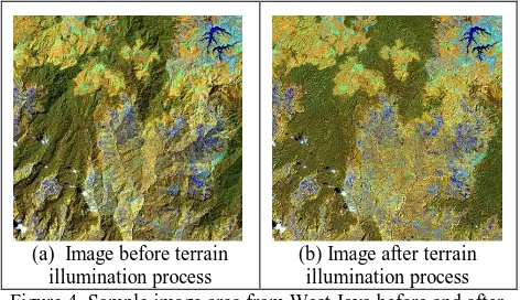
(a) Image before terrain illumination process
(b) Image after terrain illumination process Figure 4. Sample image area from West Java before and after
the terrain illumination correction. Bands 4, 5, 3 shown in RGB.
After BRDF correction, terrain illumination correction was applied to every single image. Within single image, variations in slope and aspect will result in variations in incident energy, and thus affect the reflected energy and the recorded digital number in the Landsat image. This is seen in visual images of mountainous areas (e.g. Figure 4) - slopes facing away from the sun appear darker and the slopes facing towards the sun appear brighter, even when they have a common land cover. Sun angles vary with date, so that between images from different dates (e.g. adjacent images in mosaic) these terrain illumination effects will vary in direction, location and magnitude. It is essential to correct for these terrain illumination effects before attempting to apply a numerical land cover classification to imagery from mountainous areas.
The mathematical method to perform terrain corrections is described in Wu et al (2004); it implements a modification of the C-correction of Teillet et al (1982). If the angles (slope and aspect) of the surface for each pixel are known, and correction coefficients for the land cover type are known or can be estimated, correction can be applied. Slope and aspect are derived from the DEM.
3.1.4 Cloud masking: Cloud cover is a major problem for applications using optical imagery in Indonesia and other tropical regions. It was a major concern from the initial planning stages. Dense cloud cover obscures the land and makes the affected pixels unusable for land cover mapping. Thin cloud, cloud shadow and haze affect the digital reflectance from the land cover and make quantitative processing impossible.
In order to create a composite mosaic with the maximum cloud-free land area, all cloud-, haze- and shadow-affected pixels must be removed. Methods were required to identify and remove such pixels from Landsat scenes.
The approach taken was to examine international research and best practice, to test and adapt these approaches to develop an effective method. The development of the current method has been conducted by LAPAN, with input from CSIRO and Professor Matthew Hansen (University of Maryland). The current approach is a combination of automated steps and manual refinement (digitising). The method has been developed and refined within the program in a process of continuous improvement to maximise accuracy and efficiency.
3.1.5 Mosaicing: The mosaic process produces a composite of all images within a fixed spatial extent for each year. These mosaic units form the basis for subsequent processing and products. Mosaicing can start when cloud masking of all images within the mosaic area for a year is completed. Within the mosaic process, multiple cloud-masked images within each path/row for that year are composited. The result is a single image, the ‘mosaic image’ for that year, covering the specified extents with minimum missing data.
3.2 Forest Extend and Change Mapping
There are three steps to making the annual forest extent and change products from the image mosaics. Firstly ground-truth data – expert knowledge and high resolution images – are used to associate the image signals with forest and not forest cover to create a forest base for a single year in a very hands-on approach. Then a semi-automated matching process is used to ‘match’ the data for other years to the base. In the final step, knowledge of the temporal growth patterns in forest and non-forest cover types is used in a mathematical model to refine the single-date results to provide more reliable change detection.
3.2.1 Forest base mapping: The first stage is the creation of a ‘forest base’ probability image for a chosen single year. In this stage, a ‘first’ forest probability map is created using supervised classification methods applied to the mosaics for that year. The process requires expert input to advise on land cover, and application of statistical procedures to derive the classified forest probability map. Operator judgment is used to evaluate and refine threshold parameters in the image classification process. The statistical procedures are essentially multivariate discriminate analyses; in particular canonical variate analysis (CVA) and related procedures. CVA is described in Campbell and Atchley 1981; and further described in applications using image data in Caccetta et al 2007, Furby et al 2010.
In this stage, at least three years of mosaics were required to be completed prior to the base mapping; typically mosaics for 2008, 2006 and an earlier year (2000 or 2001) were available. Year 2008 was generally the desired choice as it was close in date to most of the high resolution images.
cannot successfully separate all these different land cover types simultaneously. The classifier can then be directed (by analysis) to separate the forest and non-forest cover types which occur within that region; e.g. dryland forest and dryland non-forest land uses, or coconut palms from mangrove and wetland forests, or rice crops from wetland forest.
Forest base probability was derived by deriving indices for separating forest and non-forest cover. Indices - linear combinations of the Landsat image bands for separating forest and non-forest land covers - are optimised locally for each stratification zone. The index derivation process is driven by ground truth information – sample areas of forest and non-forest vegetation cover are selected from the image mosaic of the base year using ground truth information. Comprehensive samples of forest and non-forest cover are required within each stratification zone. Ground truth data includes high resolution satellite imagery (1-2m resolution) in which tree and non-tree cover is evident.
3.2.2 Matching: forest classification for other years: Following the base mapping, a semi-automated matching process is applied to the image mosaics to derive forest cover probabilities for the other years. As described above, the indices used in the base mapping are developed by analysis; which typically considers more than one year. In the automated matching, it is assumed that the derived indices can be applied to their zone in all years – the matching process is run to set appropriate thresholds for each of the years, which can be applied to produce the classification for that year. The matching process is applied in the Australian forest monitoring system (Caccetta et al. 2007, 2013); it has advantages of efficiency, of removing operator judgement and maintaining temporal consistency. Occasionally the automation does not produce adequate results and some manual adjustment of thresholds is required.
3.2.3 Multi temporal classification: The individual year classifications of forest probabilities are combined and refined in this stage using a mathematical approach which combines the entire time series of probabilities, along with probabilistic weights relating to accuracy, temporal change and each pixel’s neighbouring probabilities. The output is a second set of probability images, the final forest probabilities, which can be thresholded and differenced to provide extent and change maps. Models which describe probabilistic relationships between data of this kind are known as Bayesian networks. Conditional probability networks (CPNs) are used to perform the multi-temporal processing. The CPN provides a computational framework to combine uncertain data (relative likelihoods derived from satellite image data from individual years). CPNs allow for the assessment and propagation of uncertainty from multiple sources of data of varying quality or accuracy (Caccetta, 1997). The scheme for combining data was based upon techniques presented by Lauritzen and Spiegelhalter (1988) and Lauritzen (1992).
A key concept in using a multi-temporal processing scheme is that trees take time to grow. A forest cannot grow and be harvested in only one year, or even two or three years. If the spectral signal is similar to forest in one year, but not the year before nor the year after, it is unlikely to be forest. If a region is truly forest it will be forest for many years. It may stay forest (always high forest probability) or be cleared for another land
use (a sequence of high forest probabilities followed by a sudden change to a sequence of low or zero forest probabilities).
3.3. Review of Products
The final step in the processing is to review the products, both to gain feedback on their accuracy and to understand their strengths and limitations for particular purposes. This review can suggest strategies for improving the products in the future.
4. RESULT AND DISCUSSION
4.1 Results
The final results required are maps (or masks) that are indicators of forest extent at each year, and forest loss (clearing) and forest gain (revegetation) between successive years. The time series of probabilities are processed together to produce these products as binary raster maps; coded as (1) or (0). In the conversion process, thresholds are applied to each year’s probabilities to produce the extent map and differencing of these results to produce the annual change products. It is noted here that the CPN processing fills almost all areas where data were missing in the mosaics.
The key results created are:
Forest extent maps for each year (2000, 2001, ..., 2012) Forest loss and gain maps for each annual period
(2000-2001, 2001-2002, ..., 2011-2012) Year of first forest loss and gain
4.1.1 Annual Forest Extent: Forest extent was the initial result of forest monitoring. There is a forest extent result for each year of 2000-2012. Figure 5 shows the 2012 forest extent product for Indonesia.
Figure 5. Illustration of forest extent (2012) at national scale.
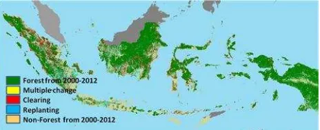
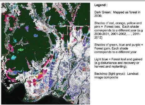
4.1.2 Annual forest loss and gain: Forest loss (clearing or harvesting) and forest gain (regrowth or replanting) results are produced for each annual interval in the time series, e.g. 2000-2001, 2001 – 2002. This can be displayed as total forest change over a number of years as in Figures 6.
Figure 6 shows the total forest loss and gain in the certain period. Dark green indicates areas that were always forest from 2000 to 2012, red shows forest loss between 2000 and 2012 while yellow indicates forest gain in the same period.
The region shown in Figure 7 is in the Central Kalimantan province, green is forest in 2002, red is forest loss from 2002 to 2003 and yellow is forest gain from 2002 to 2003. The background colour is non-forest.
Figure 7. Forest loss and gain for 2002-2003 at local scale.
4.1.3 Year of first forest loss and gain: This product identifies the year of first change in forest cover within the time series. It was developed specifically for the carbon accounting stage of the INCAS program. In the forest gain product, it provides a planting date for new plantations or a regrowth date for disturbed forest. In the forest loss product it provides a year of disturbance. Deciding whether the date is the first disturbance of natural forest or the harvest date of already disturbed forest or a plantation requires some outside knowledge of the state of the forest at the beginning of the time series.
Figure 8. Year of first forest loss and gain at regional scale coloured by year of change as indicated in the legend above.
4.1.4 Statistical summaries: The area of forested land or forest extent change can be calculated from the products and presented in tabular and graph formats. These summaries can be made at national, regional and local levels as shown in Table 1.
Time Period Forest Loss (hectares)
Forest Gain (hectares)
2000-2001 216818,75 172493,25
2001-2002 480149,25 269738,50
2002-2003 533950,75 350196,50
2003-2004 493195,50 404987,75
2004-2005 502777,50 472507,50
2005-2006 658834,75 366878,75
2006-2007 627220,00 411443,25
2007-2008 757981,25 408872,75
2008-2009 698495,25 335835,75
2009-2010 637742,75 247997,25
2010-2011 469736,50 241922,25
2011-2012 419005,50 124555,25
Table 1: Sample Forest Change Summary for Sumatra
4.2 Discussion
4.2.1 Product review discussion: A key element of any mapping program is the accuracy of the maps produced. Understanding of accuracy, uncertainty and error is critical for use of maps in different policy contexts. Understanding of error also may feed back into a continuous improvement process. Combining ground knowledge and the image processing experience which generated the products, fulfils the continuous improvement. The accuracy issues recognised during the review process are discussed below. They relate to problematic cover types (palms, wetlands, shrubs, deciduous forest, some forest management practices) where operational solutions are suggested.
Young palms are spectrally separable from forest cover types in the Landsat image data, but the spectral signal of mature palms typically becomes more like the spectral signal of some of the true forest. This is essentially a limitation of the current products.
In the wet season when wetlands are full of water, the spectral signal is very different to forest. In the dry, when the surface is bare of water, the spectral signal is also very different to forest. In between these two times, the cover is often green vegetation (grasses or reeds) growing in shallow surface water. This particular mixture of green vegetation and dark water signals appears very similar to the spectral signature of wetland forest types. What makes the forest different to wetlands is that the spectral signal from the wetland forest is relatively constant from year to year and from season to season but the signal of the other wetland vegetation varies from season to season and year to year.
artificial separation, this strategy is effective. Where there is a continuum of cover from trees to shrubs, a choice is made to map the area as either forest or not forest depending on which minimises the error in the overall forest extent.
Deciduous forests lose their leaves during some part of the year. In Indonesia such species usually lose their leaves during the dry season. This occurs with teak (jati) forests, predominantly in the eastern half of Java and other species in eastern Java, Bali and parts of Nusa Tenggara and Maluku. If imagery is captured during the dry season, there is little or no canopy and the majority of the signal is from the ground below the tree. The signal is very unlike forest. In the wet season, there is full canopy cover and a strong forest signal. As several image dates are required to build cloud-free composite images within each year, there is limited ability to select seasonally-consistent image dates. Local knowledge has been used to create stratifications zones that separate deciduous forest from other forest types. Within these zones we try to use the understorey signal to map deciduous forest as forest even in the dry season. Even with these strategies, the amount of false change mapped is higher in deciduous forests than in non-deciduous forests.
There are two main examples of forest management practices affecting the accuracy of the forest extent and change mapping. The first example is teak (jati) forest management. The quality of the wood depends on the amount of sunlight it receives. Trees are planted further apart to minimise the shadow of one tree falling on another tree, decreasing canopy density in a plantation. The ground beneath and between the trees is used for other agricultural crops, further confusing the signal received. Combined with the deciduous nature of the teak forests in some regions, these forests are difficult to map consistently. There are errors in both forest extent and change in such forests. Stratification zone boundaries are used to separate these forests from other cover, but the recommended solution is to seek or develop an independent teak forest extent map. As a very high value timber resource, information on its extent is likely to be available. Depending on quality and currency, such a map may be used to mask false change rather than adjusting the forest extent.
4.2.2. Future directions: By the middle of 2014, annual forest extent and change products for Indonesia from 2000-2012 have been produced. The effort to initiate the program and to process this historical data has been considerable, but from the middle of 2014 the program will move to a single-year ‘annual update’ mode where much less effort is required. Discussions around extending the time series back to 1990 are ongoing.
The technical capacity and data streams exist to continue the annual updates of forest monitoring into the future. Technical challenges of new data sources, such as Landsat 8 imagery, are being addressed. Insitutional support is equally important for continuity of the program – it is important that a clear mandate for the forest monitoring exists and key to this will be an evident strong demand from stakeholders for the generation of credible land cover change products.
Resourcing levels to perform an annual update (the process of adding one year sequentially to the time series) can be estimated based on recent milestone progress in the forest
monitoring. An experienced team of around six staff should be able to complete an annual update within six months.
As well as routine update activities, an ongoing forest monitoring should involve continuous improvement activities in a research component. This will include activities to evaluate new methods and to incorporate new data, and possibly to examine distribution of products in different forms. It will include research aimed at improving the accuracy of the products and at improving the efficiency of creating the products.
In parallel with improving the methodology, the infrastructure for data processing, data archiving and data delivery should be reviewed. Substantial improvements in technology have already been adopted through developments in LAPAN’s Remote Sensing Technology and Data Centre. Multi-CPU blade server computational technology has become available for the most computationally intensive steps in the processing and the data archive is being transferred to new, faster servers in the Data Centre.
Finally, the LAPAN team now has the capability to consider developing new products to complement the current forest extent and annual change maps. Such developments must be undertaken in collaboration with the other stakeholders, and will typically involve other data in addition to remote sensing
CONCLUSIONS
Annual forest extent and change products for Indonesia from 2000-2012 have been produced. The technical capacity, data streams, and the data processing infrastructure exist to continue the annual updates into the future. Technical challenges will be assessed and the current methodologies will be improved for processing new data sources, such as Landsat 8 imagery and SPOT 6 image data that have been acquired through LAPAN ground station.
Continuous improvement activities in a research component have to be considered. It will include research aimed at improving the accuracy of the products and at improving the efficiency of creating the products. Research tasks will be designed to develop and test new methods against the current results for both accuracy and efficiency. This cycle of evaluating, testing and improving can be continued throughout the program life.
ACKNOWLEDGEMENTS
and training, and other international experts have provided valuable input.
REFERENCES
Caccetta, P. A., Furby, S. L., O’Connell, J., Wallace, J. F. and Wu, X. (2007). Continental Monitoring: 34 Years of Land Cover Change Using Landsat Imagery. Paper presented at the 32nd International Symposium on Remote Sensing of Environment, June 25-29, 2007, San Jose. Costa Rica.
Caccetta P.A. 1997, Remote sensing, geographic information systems (GIS) and Bayesian knowledge-based methods for monitoring land condition. Ph.D. thesis. School of Computing, Curtin University of Technology, Perth, WA, Australia.
Caccetta, P.A. Furby, S.L, Wallace, J.F., Wu, X, Richards, G., and Waterworth, R. 2013. Long-Term Monitoring of Australian Land Cover Change Using Landsat Data: Development, Implementation, and Operation. In: Achard F. & Hansen M.C (eds). Global Forest Monitoring from earth Observation, chapter 13. Taylor & Francis. New York.
Campbell, N.A., and Atchley W.R. 1981. The geometry of canonical variate analysis. Syst. Zool. 30(3): 268-280.
Danaher, T., Wu, X. and Campbell, N. A. (2001). Bidirectional Reflectance Distribution Function Approaches to Radiometric Calibration of Landsat TM Imagery. In: Proceedings of the International Geoscience and Remote Sensing Society Symposium, Sydney, Australia, July 2001.
Furby, S.L. 2002. Land Cover Change: Specification for remote sensing analysis. National Carbon Accounting System Technical Report 9. Australian Greenhouse Office, Canberra.
Furby, S.L, Caccetta, P.A. and Wallace, J.F. 2010. Salinity Monitoring in Western Australia using Remotely Sensed and Other Spatial Data. J Environ. Quality, 39, pp16-25.
Gutman, G., Byrnes, R., Masek, J., Covington, S., Justice, C., Franks, S., and Headley, R.. 2008. Towards Monitoring Land-cover and Land-use Changes at a Global Scale: The Global Land Survey 2005. Photogrammetric Engineering & Remote Sensing, January 2008.
LAPAN. 2014. The Remote Sensing Monitoring program of Indonesia’s National Carbon Accounting System: Methodology and Products, Version 1. LAPAN_IAFCP. Jakarta.
http://pusfatja.lapan.go.id/files_uploads_ebook/pedoman/INCA
S-LAPAN remote sensing.pdf)
Lauritzen, S.L. 1992. Propagation of probabilities, means and variances in mixed graphical association models. Journal of the American Statistical Association. 87(420):1098-1108.
Lauritzen, S.L., and D.J. Spiegelhalter. 1988. Local computations with probabilities on graphical structures and their application to expert systems. Journal of the Royal Statistical Society. Series B 50(2):157-224.
Teillet, P.M., Guindon, B., Goodenough, D.G., 1982, On the Slope-Aspect Correction of Multispectral Scanner Data, Canadian Journal of Remote Sensing, 8(2), 84-106.
Townshend, J. R. G., C. O. Justice, W. Li, C. Gurney, and J. McManus, 1992. The impact of misregistration on the
detection of changes in landcover. IEEE Transaction on Geoscience and Remote Sensing, 30:1054–1060.
Tucker, Compton, J., Grant, Denelle M., and Dykstra, Jon D. (2004). NASA’s Global Orthorectified Landsat Data Set, Photogrammetric engineering and Remote Sensing, Vol 70, No. 3, March 2004, pp.313-322.
USGS 2009, Global Land Survey, 2000, Landsat ETM+, USGS, Sioux Falls, South Dakota.
Vermote, E., D. Tanré, J. L. Deuzé, M. Herman, and J.J. Morcrette, Second Simulation of the Satellite Signal in the Solar Spectrum (6S), 6S User Guide Version 0, April 1994.
Wu, X., Furby, S. and Wallace, J.F. 2004. An approach for terrain illumination correction. In: Proceedings of the 12th Australasian Photogrammetry and Remote Sensing Conference. Fremantle Western Australia.