isprs archives XLI B3 43 2016

(1)

POSE ESTIMATION AND MAPPING USING CATADIOPTRIC CAMERAS WITH

SPHERICAL MIRRORS

Grigory Ilizirov and Sagi Filin

Mapping and GeoInformation Engineering Technion - Israel Institute of Technology, Haifa, 32000

sguyalef,filin@technion.ac.il

Commission III, WG III/1

KEY WORDS: Close Range Photogrammetry; Catadioptric cameras; Pose estimation; Spherical mirrors

ABSTRACT:

Catadioptric cameras have the advantage of broadening the field of view and revealing otherwise occluded object parts. However, they differ geometrically from standard central perspective cameras because of light reflection from the mirror surface which alters the collinearity relation and introduces severe non-linear distortions of the imaged scene. Accommodating for these features, we present in this paper a novel modeling for pose estimation and reconstruction while imaging through spherical mirrors. We derive a closed-form equivalent to the collinearity principle via which we estimate the system’s parameters. Our model yields a resection-like solution which can be developed into a linear one. We show that accurate estimates can be derived with only a small set of control points. Analysis shows that control configuration in the orientation scheme is rather flexible and that high levels of accuracy can be reached in both pose estimation and mapping. Clearly, the ability to model objects which fall outside of the immediate camera field-of-view offers an appealing means to supplement 3-D reconstruction and modeling.

1 INTRODUCTION

Digital imaging makes photogrammetry relevant for a wide va-riety of applications. Yet, the limited field of view imposes lim-itations on scene coverage and necessitate acquisition of a large amount of images, even for a modest scenes. In this regards, expansion of the field of view by incorporation of or imaging through mirrors (aka catadioptric cameras) can facilitate map-ping of otherwise unseen or occluded objects or object parts. The literature also shows a broad spectrum of cameras which differ from one another by the mirror shape and their number (Gluck-man and Nayar,2001;Yi and Ahuja,2006;López-Nicolás and Sagüés,2014;Jeng and Tsai,2003;Geyer and Daniilidis,2002; Luo et al.,2007).

Such imaging configurations broaden the field of view, but are governed by light reflection from the mirror surface. Thus, the collinearity relation that stands at the core of photogrammetric modeling does not hold here any longer. The challenge is there-fore to establish object- to image-space relation in a manner that can lead to estimation of the camera pose parameters and to the performance of mapping. Our focus in this paper is on an imag-ing system which incorporates a camera and a spherical mirror. The latter is inexpensive and simple to manufacture thereby mak-ing it attractive to incorporate (Ohte et al.,2005). Its symmetric form also makes it advantageous from a modeling perspective. In terms of system modeling,Ohte et al.(2005) model the re-flection and projection of an object-point from spherical mirrors. The focus lies on the image formation rather than on pose esti-mation.Micuˇsık and Pajdla(2003) propose an approximation to the central perspective model with a single calibration parame-ter. However, the approximation error does not allow to estimate the mapping error as a function of the image noise. Lanman et al.(2006) describe a system composed of an array of spherical mirrors which provides multiple views from a single image. The authors propose a bundle adjustment-like solution, however fail to discuss accuracy matters. Agrawal(2013) uses a co-planarity constraint, based on the fact that an object-point and the sphere-and camera-centers are co-planar. Geometrical properties within

the plane are not considered there, and the sphere-center and cam-era parameters require eight or more control-points for the param-eter estimation.

In this paper we propose a novel model for pose estimation and reconstruction while imaging through a spherical mirror. Doing so, we first develop expressions that relate object- and image-space points and then model the imaging system as a whole. Our derivations yield a closed-form equivalent to the collinearity prin-ciple, which we then show that can be developed into a linear one. Studying the requirements for estimating the imaging system pa-rameters shows that a minimum of only three control-points is needed and that estimates are stable and accurate. The paper then studies reconstruction models and evaluate their accuracy. Thus, it offers not only study of the system geometry and its implica-tions on modeling and accuracy, but also provides a viable frame-work for pose estimation and modeling.

2 SPHERICAL IMAGING CONFIGURATION MODELING

Geometric relations within spherical catadioptric systems– Im-ages acquired by catadioptric-cameras are formed by reflection of light from the mirror surface and onto the image plane (Fig.1). The law of reflection states that the incident ray−−→ximi, the

re-flected ray,−−→mic, and the normal to mirror surface are coplanar

(2)

camera-axisis the vector−→oc, which links the perspective- and camera-centers, withµthe distance betweenoandc(Fig.1).

c

Figure 1. Geometry of the image formation using catadioptric spherical camera, with focus on the plane of reflection

The parameters we model in this setup, include: the camera pro-jection centerc(Fig.1) and the spherical mirror center,o. The objective is to estimate these parameters using a set of reference-points, xi, which are projected onto the image plane from the

sphere surface.

2.1 Geometric quantities of planes of reflection

In order to express the relation between a control-point, its pro-jection onto the image plane, and the direction of the extended ray, we derive first expressions that relate to both the axial camera configuration and the reflection of light from the sphere surface. These consist of four elements within theplane of reflection, and include: i) the angleγibetween the camera-axis,−→oc, and−−→mic;

ii) the distancedi, between the projection center,candqi, the

point at the intersection of the extended ray−−→ximiwith−→oc;iii) the

angleδi, between−→ocand the normal to the sphere’s surface; and

iv) the angleφi, between−−→xiqiand

− →_oc

(Fig.1). To keep the model applicable to any type of central camera (e.g., one equipped with a fish-eye lens), we use angular quantities which are measurable in the image reference frame.

Computingγi, requires first to define the image-space direction

of−→oc. This direction must be estimated as the mirror’s center,o, does not show on the image. We make, first, a reference to meth-ods that are based on either placement of actual markers on the lens or projection of the sphere’s boundary onto the image fol-lowing the camera orientation (Kanbara et al.,2006;Francken et al.,2007). However, we develop an alternative one that requires neither, and which is valid for any central camera.

We begin by observing that the projection of the mirror boundary on the image, relates to the tangent ray to the sphere’s surface,−mc→ (Fig.1), suggesting that the angle,α, between these two vectors remains the same for any point on the boundary, and thus:

vTi−→oc=kvikk−→ockcos(α) (1)

withvithe image space direction towards sphere boundary. As

our interest is only in the direction of−→oc, we set:

k−→ock= cos(α)−1

(2)

and so can write:

vTi−→oc=kvik (3)

which can then be extended to multiple observations and allow to estimate−→oclinearly and thereby compute the angleαby Eq. (2). The angleγican then be computed by the scalar product between

− →

ocand−−→cmi. Additionally, as the radius vector is perpendicular to

the tangent ray (Fig.1), we also have that:

sin(α) = r

µ (4)

suggesting both that the ratior/µis constant and known, and that ifris known,µcan be derived.

We can now derive expressions for the following quantities within theplane of reflection:i) the angleγibetween−→ocand−−→mic,ii) the

distancedi, from the projection center,c, to the intersection of

the extended ray−−→ximiwith the camera-axis atqi,iii) the angle

δi, between−→ocand the normal to the sphere’s surface, andiv) the

angleφi, between−−→xiqiand−→oc(Fig.1).

The angleγiis the scalar product between−→ocand−−→cmiand the

following three quantities are given by (cf. the Appendix for their derivation):

These geometric quantities describe both the reflection of a point onto image space and the direction of−−→ximi, the extended ray,

for any plane of reflection. The relation between two planes of reflections is given by a rotation,ψijabout the−→oc, which is given

by:

cos(ψij) =

cos(ξij)−cos(δj)cos(δi)

sin(δj)sin(δi)

(8)

whereξijis the angle between two planes of reflection, and whose

derivation is given inIlizirov and Filin(2016).

via which the angleψijbetween the two plane of reflection is

de-rived and, together with the plane of reflection derivatives, define the axial camera.

2.2 Transformation between the plane of reflection and object-space

To establish the relation between the planes of reflection and object-space, we introduce an intermediate coordinate system, M, whose center lies atc, itsx-axis is−→oc, itsy-axis is orthog-onal to thex-axis on an arbitrary plane of reflection (e.g., on that containingx1), and thez-axis completes a right-hand-side

(3)

wherevirepresents the rotation around−→oc, andwithe line slope

in the plane of reflection. The angleviis derived fromψij, and

the parameterwican be derived fromφi(Fig.1) by:

The transformation from theMsystem to object-space is of Eu-clidean nature.1Therefore:

[x]M =RT(x−c) (12)

wherecis the camera perspective center, andR= [r1 r2 r3]

is the rotation matrix whose columns are:

r1=

Finally, use of Eq. (12) and Eq. (9) allows writing:

RT(xi−c)−[qi]M =ui[pi]M ⇒

which provides an equivalent to the colinearity relation, where a point in object-space,xi, is linked to derivable image-space

quan-tities (here,φi,diandvi). Similar to central perspective cameras,

collineation is of the control-point-to-projection-center direction in both image- and object space. From Eq. (14) the rotation an-gles inRand the camera position,ccan be derived directly. To derive the mirror’s center,o, we use:

o=c+µr1=c+r

Parameters estimation using DLT– Notably, and while not elabo-rated here, our representation (Eq.14) facilitates linear modeling of the system. By dividing thelasttwo rows by the first, the pa-rameterucan be eliminated, thereby and equivalent form to the DLT. Its appeal lies in the direct estimation without the need for first approximations or iterations.

2.3 Mapping

Using two or more images can be used to estimate position of a point in object-space. Using Eq. (9), we describe the rays towards xin twoM-systems for a point that appears in two images (M1

andM2, respectively) by:

[x]M₁=u1[p1]M₁+ [q1]M₁ (16)

[x]M₂=u2[p2]M₂+ [q2]M₂ (17)

1

Under the assumption that the radius is given.

whereu1andu2are unknown scalars. Using the estimated model

parameters, each of the rays can be transformed into object space:

ei=Ri[qi]Mi+ci (18)

si=Ri[pi]Mi (19)

yielding:

x=u1s1+e1 (20)

x=u2s2+e2 (21)

which form two lines in object space that intersect inx. We have six equations and five unknowns, (x,u1andu2) and the point can

be estimated by least-squares adjustment.

3 ANALYSIS AND RESULTS

Having established the parameter estimation models, their perfor-mance is now analyzed. The analysis is carried out over different control configurations, at different levels of noise.

The model is tested using both simulated experiments, under re-alistic imaging configurations, and real-world data. The imag-ing system consists of a standard pinhole camera and a spherical mirror, where the camera intrinsic parameters are assumed to be calibrated in advance. Parameters similar to the real-world exper-iments were used for the synthetic tests, with:µ= 500mm, and r= 74mm.

3.1 Influence of control point configurations on the param-eter estimation

To test the quality of the estimation and the influence of the control-point distribution, we observe that the distribution of control-points in image-space has the greater influence on the solution (cf. Sec.2.2). Thus, we describe the points by their angular image-related quan-tities: vandγ. Three different configurations are evaluated: i) a random distribution of points; ii) an X-shaped arrangement, which represents an even distribution of the angleγ; andiii) a circular arrangement of points, which represents an even distri-bution of the anglev(Fig.2). In reference to the necessary num-ber of control points, the resection model (Eq.14) yields three equations which include an unknown scale factor. Therefore, only three control points are needed to estimate the six positional parameters. To ensure sufficient redundancy and distribution in image-space, 20 control points are used in each experiment. All models are tested with noise levels ranging fromσ= 0.1to1.5 pixels. Accuracy estimates of the model parameters are the mean of 100 trials for each noise level.

Applying theresectionmodel for therandompoint distribution (Fig.2a) yields sub-millimeter accuracy estimates for 0.5 pixels noise or lower; lower than 2 mm estimates for a 1 pixel noise level, and lower than 2.5 mm for a 1.5 pixels noise-level (Ta-ble1). The condition number ofGrammianmatrix is 830. No-tably, throughout the analysisσXof the mirror is omitted as the

camera-mirror position along the central-line is related by the dis-tanceµ, which is computed in advance as a function ofα(Eq.4). The angleαis the outcome of a separate adjustment process, and being accurately estimated, its influence on the accuracy ofµ is negligible. As an example, for a 1 pixel measurement noise, σα = ±1×10−

4

rad which translates toσµ = ±0.01mm for

(4)

(a) Random arrangement (b) Evenγarrangement

(c) Evenvarrangement

Figure 2. Three control configurations. Each configuration con-sists of 20 points

Noise Camera position [mm] Mirror position [mm] σ[pix.] σX σY σZ σY σZ

0.1 0.03 0.16 0.14 0.06 0.06 0.2 0.07 0.36 0.29 0.12 0.11 0.5 0.17 0.86 0.74 0.31 0.33

1 0.38 1.63 1.39 0.53 0.59

1.5 0.54 2.86 2.26 0.88 1.05

Table 1. Parameter accuracy measures as a function of the noise level, using random point distribution (Fig.2a)

σ[pix.] σθ[deg] σd[mm]

0.1 0.01 0.01

0.2 0.01 0.02

0.5 0.04 0.05

1 0.07 0.11

1.5 0.11 0.15

Table 2. Accuracy measures for the position and orientation esti-mation of the central-line

TheX-shaped point arrangement offers an even distribution inγ along two planes of reflection (Fig.2b).2Estimates for the resec-tionmodel are listed in Table (3), showing some improvement in the accuracy but not on a significant level, with a nearly similar condition number 832.

0.1 0.04 0.13 0.13 0.06 0.06 0.2 0.08 0.28 0.27 0.12 0.12 0.5 0.21 0.76 0.71 0.34 0.32

1 0.47 1.43 1.40 0.62 0.58

1.5 0.69 1.90 2.20 0.72 0.94

Table 3. Parameter accuracy measures as a function of the noise level, usingX-shaped arrangement (Fig.2b)

2

As a solution cannot be obtained using a single plane of reflection, this configuration is the minimal distribution ofv.

Thecircularpoint arrangement offers fixedγvalues and an even distribution inv(Fig.2c). Accuracy measures for theresection model are somewhat higher than the previous two, but not on a significant level (Table4), while the condition number dropped to 103.

0.1 0.02 0.08 0.07 0.04 0.04 0.2 0.05 0.17 0.16 0.08 0.08 0.5 0.12 0.42 0.48 0.22 0.25

1 0.27 0.82 0.97 0.47 0.52

1.5 0.37 1.29 1.45 0.77 0.78

Table 4. Parameter accuracy measures as a function of the noise level, using two circles arrangement (Fig.2c)

These results show that as long as the point distribution is spread throughout the image their arrangement has a lesser effect on the pose estimation. The correlations among the estimated param-eters is not extreme. However, relatively high correlations can be observed between theY and between theZ values (∼88%). Analysis of the rate of convergence shows similar patterns to those of the conventional central projection model.

3.2 Real world experiment

Testing the model on real world data, a spherical mirror was placed inside a box with three surrounding vertical planes cov-ered by a checkerboard pattern. Measurement of the camera pose with the checkerboard related control points, and when reflected from the sphere surface was carried out. While not listed here, accuracy equivalent to the results obtained by the simulated test were reached. These results suggest that the proposed model re-flects indeed the real-world settings.

3.3 Mapping

Finally, and as noted in Sec.2.3, once the camera and mirror position are estimated, mapping can be performed by intersection of the extended rays−→q1xand

−→

q2x(Eqs.20;21). In that respect,

the intersection of the extended rays with the camera axes ate1

ande2, is equivalent to the central perspective baseline, which

here becomeske1e2k(Fig.3).

With this observation in mind, and with the understanding that higher accuracy can be reached with wider baselines (ke1e2k),

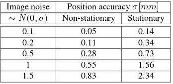
we study two mapping scenarios: the first is the conventional one, in which two images are acquired through a stationary mirror; and the second is designed so that the baseline is extended. For this, we not only move the camera but also the spherical mirror between acquisitions (Fig.3b).

To test the expected accuracy of both settings, we study a setup in which two images are acquired with a distance ofkc1c2k =

770mm between them, but where the mirror is also shifted by k−−→o1o2k = 280mm in second setup. Comparing the baseline

under both setups show that in the first oneke1e2k is

(5)

∆θ= 45◦_(∼₁₅◦_vs.₆₀◦_{) and leading to a less accurate} recon-struction. This is expressed in Table (5) for varying noise levels. The accuracy of the stationary scenario is two-fold lower than that obtained by the second scenario.

o

c1

c2

x

e1 _e

2

θ

(a) Stationary mirror

o1 o2

c1

c2

x

e1 _e₂

θ

(b) Two mirrors

Figure 3. Mapping using reflection from spherical surfaces

Image noise Position accuracyσ[mm] ∼N(0, σ) Non-stationary Stationary

0.1 0.05 0.14

0.2 0.11 0.34

0.5 0.28 0.73

1 0.55 1.56

1.5 0.83 2.34

Table 5. Estimated position accuracy measures as a function of the noise level

4 CONCLUSIONS

The paper studied pose estimation and mapping from a catadiop-tric system that consists of a camera and a spherical mirror. As demonstrated, this system forms an axial camera where all ex-tended rays intersect at an axis linking the camera’s perspective center and the sphere center. Notably, the system remains ax-ial irrespective of the relative position or orientation between the camera and sphere. Through derivation of measures within and then between planes of reflection a closed form similar to the collinearity principle has been derived, which was then extended into a linear model. Further analysis of the system’s geometry has

led to an alternative, trilateration-based model that yielded bet-ter estimates and proved robust to outliers. Results and analysis show that as long as the control configuration does not introduces degeneracies, high-levels of accuracy can be reached in estimat-ing the pose parameters. Furthermore, the system radius can be calibrated, even at sub-millimeter level of accuracy. Evaluation of the reconstruction with this system has managed to draw resem-blance to central perspective cameras, thereby applying known principals in assessing the reconstruction accuracy. This has led to an alternative modeling approach that helps both broadening the ‘imaging’ baseline thereby having high accuracy levels.

REFERENCES

Agrawal, A., 2013. Extrinsic camera calibration without a direct view using spherical mirror. In: Computer Vision (ICCV), 2013 IEEE International Conference on, pp. 2368–2375.

Francken, Y., Hermans, C. and Bekaert, P., 2007. Screen-camera calibration using a spherical mirror. In: Computer and Robot Vision, 2007. Fourth Canadian Conf., IEEE, pp. 11–20.

Geyer, C. and Daniilidis, K., 2002. Paracatadioptric camera cali-bration. IEEE Transaction on PAMI 24(5), pp. 687–695.

Gluckman, J. and Nayar, S. K., 2001. Catadioptric stereo using planar mirrors. Int. J. of Computer Vision 44(1), pp. 65–79.

Ilizirov, G. and Filin, S., 2016. Robust pose estimation and cali-bration of catadioptric cameras with spherical mirrors. Submited.

Jeng, S.-W. and Tsai, W.-H., 2003. Precise image unwarping of omnidirectional cameras with hyperbolic-shaped mirrors. In: Proc. 16th IPPR Conf. Comput. Vis., Graphics Image Process., Kinmen, Taiwan, pp. 17–19.

Kanbara, M., Ukita, N., Kidode, M. and Yokoya, N., 2006. 3d scene reconstruction from reflection images in a spherical mir-ror. In: Pattern Recognition, 2006. ICPR 2006. 18th International Conference on, Vol. 4, IEEE, pp. 874–879.

Lanman, D., Crispell, D., Wachs, M. and Taubin, G., 2006. Spherical catadioptric arrays: Construction, multi-view geome-try, and calibration. In: 3D Data Processing, Visualization, and Transmission, Third International Symp., IEEE, pp. 81–88.

López-Nicolás, G. and Sagüés, C., 2014. Unitary torus model for conical mirror based catadioptric system. Computer Vision and Image Understanding 126, pp. 67–79.

Luo, C., He, L., Su, L., Zhu, F., Hao, Y. and Shi, Z., 2007. Omnidirectional depth recovery based on a novel stereo sensor. ACCV’07 Workshop on Multi-dimensional and Multi-view Im-age Processing, vol. 2 issue 2.

Micuˇsık, B. and Pajdla, T., 2003. 3d reconstruction with non-central catadioptric cameras. Research Reports of CMP, Czech Technical University in Prague, No. 19.

Ohte, A., Tsuzuki, O. and Mori, K., 2005. A practical spherical mirror omnidirectional camera. In: Robotic Sensors: Robotic and Sensor Environments, 2005. International Workshop on, IEEE, pp. 8–13.

Ramalingam, S., Sturm, P. and Lodha, S. K., 2006. Theory and calibration for axial cameras. In: Computer Vision–ACCV 2006, LNCS 3852, Springer, pp. 704–713.