COMPARATIVE ANALYSIS OF DIFFERENT
LIDAR SYSTEM CALIBRATION TECHNIQUES
M. Millera, A. Habiba a
Digitial P hotogrammetry Research Group Lyles School of Civil Engineering
P urdue University, 550 Stadium Mall Dr., West Lafayette, IN 47907, USA -(mill1154, ahabib)@purdue.edu
Commission I, WG I/3
KEY WORDS: Aerial LiDAR, quality control, quality assurance, systematic errors, standard operating procedures,
AB STRACT:
With light detection and ranging (LiDAR) now being a crucial tool for engineering products and on the fly spatial analysis, it is necessary for the user community to have standardized calibration methods. The three methods in this study were developed and proven by the Digital P hotogrammetry Research Group (DP RG) for airborne LiDAR systems and are as follows; Simplified, Quasi -Rigorous, and Rigorous. In lieu of using expensive control surfaces for calibration, these methods compare overlapping LiDAR strips to estimate the systematic errors. These systematic errors are quantified by these methods and include the lever arm biases, boresight biases, range bias and scan angle scale bias. These three methods comprehensively represent all of the possible flight configurations and data availability and this paper will test the limits of the method with the most assumptions, the simplified calibration, by using data that violates the assumptions it’s math model is based on and compares the results to the quasi-rigorous and rigorous techniques. The overarching goal is to provide a LiDAR system calibration that does not require raw measurements which can be carried out with minimal control and flight lines to reduce costs. This testing is unique because the terrain used for calibration does not contain gable roofs, all other LiDAR system calibration testing and development has been done with terrain containing features with high geometric integrity such as gable roofs.
1. INTRODUCTION 1.1. Calibration and Q uality Control
System calibration is considered to be one of the activities of quality assurance (QA), and the purpose is to estimate the systematic errors which describe any physical deviation from the system’s theoretical model. The LiDAR system is composed of the laser unit, a global navigation satellite system (GNSS) unit, and an inertial navigation system (INS). Often times LiDAR system calibration is done by the data provider and is considered a trade secret, while quality control (QC), is traditionally done by the end user and is done in order to prove the completeness and correctness of the LiDAR product (Bang et al., 2010). For LiDAR, calibration and QC are not independent processes; QC can be used to improve the system calibration parameters and can be done in several different ways depending on the type of data and its availability.
Often times QC entails the use of control surfaces. Since control is expensive and time consuming to obtain, the three methods here are developed by comparing overlapping strips. The overlapping strips behave significantly different fro m each other when systematic errors (SE) and random errors (RE) are present and these errors are exposed by subtracting the strips and observing differences that are above the noise level of the data. Comparing strips has been proven to be
substantial for QC when the flight configuration is optimized to magnify and decouple the systematic errors that are inherent in multi-sensor LiDAR systems (Bang et al., 2010 ). The geometric configuration of the three sensors, GNSS, INS, and laser, are known but contain small yet significant biases that introduce error and affect the overall accuracy of the resulting point cloud. This configuration will be covered in section 3 along with additional background information.
2. B ACKG ROUND 2.1. LiDAR Math Model
The LiDAR point positioning math model is a summation of three vectors and is a function of the position, orientation, and measurements from each unit in the system.
�1 = � + ��
+ � � �1
(1)
The four coordinate systems are the mapping frame, IMU body frame, laser unit frame, and laser beam frame as seen in Figure 1. A ground coordinate is reconstructed by applying the appropriate rotations coming from the platform attitude, laser beam directions, and boresight angles (Vaughn et al., 1996). The resulting coordinate is considered the true coordinate; this equation does not include the biases of the system parameters. All derivations are based off of this point positioning equation, represented here as �1 , indicating the point I is in the mapping frame. The derivations to follow in section 4 will represent �1 as ⃗⃗⃗ for simplicity.
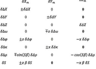
2.2. LiDAR Error Sources and their Impact Systematic and random errors are inherent in any measuring unit and more so with a system of several units that require precise alignment. The systematic errors of the LiDAR system have intuitive effects on the reconstructed object space coordinates and are shown in the Table 1.
The biases are listed in the first column and the impacts that each one has on the X, Y, and Z coordinates are found by taking the derivative of the LiDAR point positioning equation with respect to system parameters and multiplying by the biases of the system parameters (Habib et al., 2009). The biases include the three lever-arm components, three boresight
angles, bias in the range, and bias of the scan angle scale. The range bias and the bias in scan angle scale correspond to measurements while the remaining biases correspond to system parameters. Boresight biases affect planimetric coordinates more than the vertical coordinate, and the range bias mainly affects the vertical coordinate. The boresight biases are of the most concern in calibration as they are the most unstable and have the largest possible effects on the
quality of the point cloud. The Z component of the lever-arm is usually very good, but it is coupled with the bias in the range measurement. The Quasi-rigorous and Rigorous methods are able to determine the bias in the range measurement because it can only be determined through the use of external control and the simplified method does not allow the use of control (Habib et al., 2010).
Table 1: Effects of Biases on Each Component of the Reconstructed Coordinate
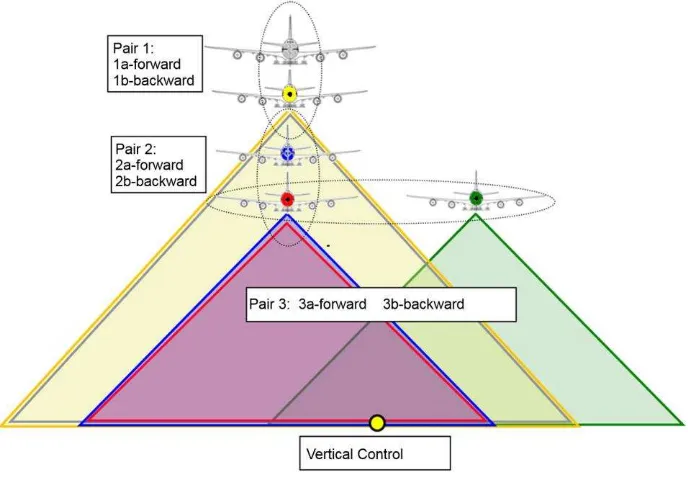
certain biases and magnifies others so that estimation of the biases is possible. There must be two pairs of flight strips going in the opposite directions, each at significantly different flying heights, and one pair of flight strips going in the same direction with a large lateral distance between them as seen in Figure 2 below (Bang et al., 2010).
The effect that the heading boresight angle bias has on the object space coordinates is detectable with the pair going in the same direction. It is also necessary that this set has a
significantly large lateral distance in order to magnify the effect of the bias in the heading boresight angle. The bias in the leverarn along the flight directions and the bias in the boresight pitch angle are highly correlated and must be decoupled by using two flying heights (Habib et al., 2010). These can be decoupled because the effect that the boresight pitch angle bias has on the reconstructed coordinates is dependent on the flying height while the other is not.
2.4. Q C Measures & ICPATCH
LiDAR data is irregular, it is not guaranteed that the same exact point will occur in overlapping scans as in photogrammetry where its positioning/reconstruction equation is based on redundancy. With irregular 3d data, corresponding points and their similarity measures are not as straight forward as other data such as photogrammetry where distinct point can be measured. Since point to point correspondences do not exist, conjugate features are heuristically approached.
Throughout the many tests on primitives, conjugate features , and their similarity measures, the most recommende d correspondence for LiDAR point cloud analysis is between discrete points in one scan and triangular irregular netwo rks
(TIN) in the other scan (Maas, 2002 ). In this study ICP atch is used with these correspondence and it outputs discrepancies between the two point clouds via optimizing the 3D rigid body transformation between correspondences, which is point to patch as seen below (Kersting, 2011).
Several other studies have been done on using features that are already in the scene as geometric constraints, such as extracted lines from gable roofs (Vosselman, 2002) or planes (P feifer , 2005). ICP atch is preferred here because is based on the
original, irregular points as input versus using lines and planes that require preprocessing on the data to locate within the point cloud. Also, planar and linear features are not always available for natural scenes.
Figure 3: ICP atch procedure
3. METHODOLOG Y
height, each pair’s two strips must be captured at the same height, and must be collected with a linear, vertical scanner. The Quasi-Rigorous has the same assumptions except it does not require parallel fight lines and there are no restrictions on the terrain height and flying height. The rigorous calibration method has no assumptions on the data or the terrain. As for the data requirements, the simplified method only requires the point cloud coordinates, the quasi-rigorous requires the time tagged trajectory and time tagged coordinates, and the rigorous requires all of the raw measurements, which entails the GNSS, INS and laser components unprocessed data (Kersting, 2011).
3.2. Models
As discussed in section 3, the LiDAR coordinates are formulated as a function of measurements, � , and system parameters, , as seen in equation 2. Adding biases, � , to the system parameters will give the biased coordinate shown in equation 3. This equation is nonlinear and can be linearized through the Taylor series expansion and excluding all higher order term, the reduced form can be seen in equation 4.
� � = ,� (2)
�� = + � ,� (3)
�� ≈ ( , � ) + � = � � + � (4)
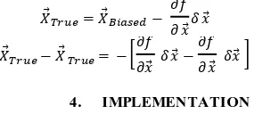
The difference of the true coordinate and the biased results in the effect the biases have on the reconstructed coordinates as seen in equation 5 below.
�� − � � = � (5)
3.3. Simplif ied Calibration Derivation
The simplified calibration assumptions reduce the point positioning equation 1, to equation 6 below. Equation 1 is in compact form and the expanded matrix form is shown here to specifically display how the assumptions simplify the point positioning equation.
The impact of the biases are found by taking the derivative of the point positioning equation with respect to the system parameters and multiplying by the biases the result can be seen in equation 8. Equation 9, the difference of the biased
The key to the simplified calibration solution is that equation 9 is reconfigured to represent a rigid body transformation. The transformation parameters are a linear combination of the biases and once they are found via ICP atch the biases are estimated with Least Squares.
3.4. Q uasi-Rigorous Calibration Derivation
The quasi-rigorous calibration assumptions reduces equation 1 to equation 10 below. The compact form is expanded to full matrix form to specifically show how the assumptions simplify the point positioning equation.
� �
The impact of the biases are found by taking the derivative of the point positioning equation with respect to the system parameters and multiplying by the biases just as we did in the simplified method. The difference of the coordinates of the conjugate points is again the basis for the solution and that is simplified to be the difference of the impacts of the biases on strip A and strip B as seen in equation 9 above. The final quasi-rigorous calibration math model does not turn out to be representative of a 4 parameter transformation as in the simplified. Instead of a linear estimation of the biases , the biases are estimated iteratively on equation 9 until some convergence criteria is reached.
3.5. Rigorous Calibration Derivation
coordinates is simplified into equation 12 below and the rigorous calibration solution iterates on a collection of these equations to report the correction.
� � = �� − � (11)
� � − � � = − [ � − � ] (12)
4. IMPLEMENTATION
The data used in this experiment was simulated by a program that emulates an airborne LiDAR system flying along the specified trajectory collecting data according to the input specifications for a certain amount of time. All possible configurations are allowed in the simulator. Using a digital elevation model (DEM) as a reference surface, the simulator determines the firing point of the laser unit and extends that ray until it intersects the DEM to calculate one point at a time. All the components of the LiDAR point positioning equation are entailed in the calculation. In addition to the starting point, system parameter values, and the internal LiDAR unit specifications, the simulation program allows for noise specifications of the measured values as input data. In this experiment we used the LiDAR specifications detailed in table 2, a DEM with terrain varying from 0 -100 m as seen in Figure 4, and incorporated noise with magnitudes seen in table 3. As mentioned previously the terrain used for this testing does not contain gable roofs or any other distinct features as seen in Figure 3.
LiDAR Specifications
P ulse Rate (pulses/s) 3.00e-05
Scan Rate (scans/s) 0.025
Laser Angle (°) 30
Table 2: LiDAR Specification Used in these Experiments
Figure 4: P ortion of DEM used in these Experiments
Noise
GP S – X, Y, Z (m) 0.05, 0.05, 0.10
INS - ,�,� " 9, 9, 18
Mirror Angle Encoder (") 3
Range (m) 0.02
Table 3: Noise of Measurements in these Experiments
5. EXPERIMENTAL RESULTS
The simplified calibration is derived with various assumptions, as described above. Some are more realistic in a real world scenario and one that may often be violated is the parallel flight lines assumption. It states that two strips that are being compared, in this case strip A and strip B, should be parallel to each other in order for the data to comply well with the derived
math model and successfully carry out the calibration. The flight lines for all six flights will be deviated from each other first with ten degrees, then twenty degrees, and finally thirty degrees. The results from the simplified calibration will be compared to that of the quasi -rigorous and rigorous methods that do not require parallel flight lines.
Figure 5 is a bird’s eye view of the flight lines. Each of the six flight lines is deviated by fifteen degrees, pair 3’s flight lines are on the outer edges while pair 1 and 2’s deviated flight lines are overlapping each other and are shown in the middle.
Figure 5: Flight Line Deviation of 30°
6. CONCLUSIONS & FUTURE WORK The simplified, quasi-rigorous, and rigorous calibration methods were developed to provide accurate and reliable methods to perform system calibration for various types of data availability at minimal costs. When no raw measurements are available, the simplified calibration can be performed with just the point cloud but it is the method with the most assumptions. This study has shown that performing calibration
with data that violates the assumptions of the simplified calibration results in a successful estimation of the biases with the exception of the difference between the scan angle scale factor simulation and estimation. Further testing will be done to see if this is due to the absence of gable roofs. Their presence helps the matching process by providing rigid geometric features, and this is the first time LiDAR system calibration testing has been done on terrain without them. These experiments further emphasize that system calibration is Table 4: Calibration Results of the 10 ° Angular Deviation
Table 5: Calibration Results of the 20° Angular Deviation
attainable and successful with no raw measurements, and with minimal flights and control. A new method is being derived that is considered a combination of the simplified and the quasi-rigorous calibration. It will be more comparable to the quasi-rigorous and rigorous calibrations than the simplified because it will be an iterative one-step procedure instead of the current two-step procedure, and will also be able to incorporate control like the quasi-rigorous and rigorous methods. This method will not also require that the two strips being compared to be captured at the same flying heights and the terrain relief with respect to the flying height will be insignificant. In addition to the development of a new calibration method, a stability analysis will be done to establish how long calibration results can be used before repeating the process.
REFERENCES
Bang, K. 2010. Alter na tive Methodologies for LiDAR System Ca libr a tion, P h.D. Dissertation, Department of Geomatics Engineering Calgary.
Bang, K., Habib, A., and Kersting, A., 2010. Estimation of Biases in LiDAR System Calibration P arameters using Overlapping Strips. Canadian Journal of Remote Sensing, Vol.
36, Suppl. 2, pp. S335–S354.
Habib, A., Bang, K., Kersting, A., and Chow, J., 2010. Alternative Methodologies for LiDAR System Calibration. Remote Sensing Jo ur na l (ISSN 2072-4292), Vol. (2), pp. 874 - 907.
Habib, A., Bang, K., Kersting, K., and Lee, D., 2009. Error Budget of LiDAR Systems and Quality Control of the Derived Data. P hotogr a mmetric Engineer ing a nd Remote Sensing, vol. 75, no. 9, pp.1093-1108.
Habib, A., Bang, K., Kersting, K., and Lee, D., 2009. Error Budget of LiDAR Systems and Quality Control of the Derived Data. P hotogr a mmetric Engineer ing a nd Remote Sensing, vol. 75, no. 9, pp.1093-1108.
Kersting, A. 2011. Qua lity Assura nce of Multi-Sensor System, P h.D. Dissertation, Department of Geomatics Engineering Calgary.
Maas H. G., 2002. Method for measuring height and planimetry discrepancies in airborne laserscanner data, P hotogr a mmetric Engineer ing a nd Remote Sensing, 68(9):933–940.
P feifer, N., Elberink, S.O., and Filin, S., 2005. Automatic Tie Elements Detection for Laser Scanner Strip Adjustment,
ISPRS W G III/3, III/4, V/3 W orkshop “Laser scanning 2005”, 12-14 September, Enschede, the Netherlands. pp. 1682 -1750.
Vaughn, C.R., Bufton, J.L., Krabill, W.B., and Rabine, D.L.,
1996. Georeferencing of airborne laser altimeter
measurements, Inter na tiona l Journa l of Remote Sensing, Vol. 17, No. 11, pp. 2185-2200.
Vosselman, G., 2002. Strip offset estimation using linear features, 3r d Inter na tiona l Wor kshop on Ma pping Geo