MAV-BASED REAL-TIME LOCALIZATION OF TERRESTRIAL TARGETS WITH
CM-LEVEL ACCURACY: FEASIBILITY STUDY
Yosef Akhtman, Abhinav Garg and Jan Skaloud
TOPO Lab, ´Ecole polytechnique f´ed´erale de Lausanne, Lausanne, Switzerland
{yosef.akhtman,abhinav.garg,jan.skaloud}@epfl.ch http://topo.epfl.ch
KEY WORDS:UAVs, MAVs, Photogrammetry, Sensor Orientation, Direct Georeferencing
ABSTRACT:
We carry out a comprehensive feasibility study for a real-time cm-level localization of a predefined terrestrial target from a MAV-based autonomous platform. Specifically, we conduct an error propagation analysis which quantifies all potential error sources, and accounts for their respective contribution to the final result. Furthermore, we provide a description of a practical MAV system using the available technology and of-the-shelf components. We demonstrate that, indeed, the desired localization precision of a few centimeters may be realistically achieved under a set of necessary constraints.
1 INTRODUCTION
The field of micro-air-vehicles (MAVs) has been recently experi-encing a surge in research and development, as well as rapid com-mercialization. The potential applications include aerial mapping, surveillance, remote sensing, support of emergency services, telecom-munications, etc. The key appeal of the MAV concept is constituted by its mobility in conjunction with the small form-factor, license-free operation, and the convenience of a single operator handling.
Despite the considerable potential, the design of MAV platforms, which would be capable of matching the functional efficacy exhib-ited by some of the larger UAVs has proven to be a major chal-lenge, largely because of the stringent constraints on the size and the weight of the on-board sensor and computing equipment (Pines and Bohorquez, 2006). A considerable progress in this context has been recently reported, for instance, in (Zufferey et al., 2010), where a high-resolution wide-area mapping and visualization have been achieved using a 500g Swinglet MAV platform, that employs of-the-shelf consumer-grade digital camera as the optical sensor. Subsequently, a relatively accurate georeferencing of the acquired visual data has been realized using a bundle adjustment method (F¨orstner and Wrobel, 2004). Nevertheless, a real-time georefer-encing of terrestrial targets with a sub-decimeter precision, rou-tinely required in some professional applications, from a MAV plat-form remains an open problem.
In this paper we discuss the design considerations for a MAV plat-form capable of a cm-level localization of terrestrial targets by the means of direct real-time localization of a predefined planar target using a combination of on-board sensors including a GPS, an IMU and a high-resolution camera. Specifically, in Section 2 we intro-duce an alternative formulation of a standard direct georeferencing problem, which utilizes thea prioriknowledge of a terrestrial tar-get’s dimensions and internal orientation. In Section 3 we conduct a comprehensive analysis of the error propagation inherent to the system design and the algorithmic flow considered. In Section 4 we provide a description of a practical MAV georeferencing system in development and detail the numerical properties of all potential noise sources associated with the various system components. Fi-nally, in Section 5 we provide a quantitative analysis of the achiev-able performance before drawing our conclusions in Section 6.
2 PROBLEM FORMULATION
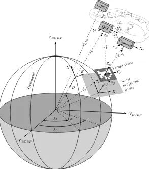
We commence with the mathematical formulation of the standard georeferencing problem, namely that of determining the position of a physical pointpin the Earth-centered Earth-fixed (ECEF) frame of reference from an airborne platform, as illustrated in Fig. 1 and described in (Schwarz et al., 1993)
xep(t) =xbe(t) +Rel(t)Rlb(t)Rsb(ωb, φb, κb)
xbs+xsp(t)
,
(1)
wherexe
b(t)is the navigation center of the onboard IMU, which
represents the origin of the body (b) frame in the earth (e) frame of reference;xb
sdenotes the relative displacement between the optical
sensor (s) and the body frames of reference origins, while the rota-tion matrixRbsdescribes the corresponding relative misalignment between thesand thebframes, and is defined by the three Euler anglesωb, φbandκb. Finally,RlbandR
e
ldenote the rotation
matri-ces, which represent the body-to-local and the local-to-earth frame conversions, respectively. The notation(t)indicates the temporal variability of the preceding quantity.
In the context of this paper, however, we would like to substitute the singular pointpwith a planar target of predefined dimension, asym-metric marking and orientation, which introduces a corresponding right-handed frame of referencephaving itsz-axis pointing up per-pendicular to the plain of the target as well as thexand yaxes predefined in the plain of the target. Furthermore, we would like to introduce the notationxkijto denote a vector from the origin of frameito the origin of framejand expressed using thekframe of reference.
Consequently, we may reformulate Eq. (1) based on the following analysis
xep(t) =xeb(t) +Rel(t)xlbp(t) =xeb(t)−Rel(t)xlpb(t)
=xeb(t)−Rel(t)Rlp(t)xp
b(t), (2)
where we have the target-to-local frame transformation
ab
Figure 1: MAV-based direct georeferencing.
and the target-to-body vector
xp
Observe that substituting (4) and (3) into (2) makes the resultant ex-pressions of Equations (2) and (1) identical. Importantly, however, the target’s position estimation expression in (2) eliminates the di-rect dependency on the quantitiesRl
b(t)andx s
p(t)which are
sub-ject to rapid temporal variability due to the instantaneous changes to the MAV’s orientation, in particular roll and pitch. Instead, in (2) we have the target-to-local frame transformationRl
p(t), which only
depends on the target’s attitude that may be assumed time-invariant and will be therefore denoted as simplyRlpfrom here on; as well as the target-to-body vectorxp
b(t), which has to account for the
rela-tively slow translational movements of the MAV, but is independent of its orientation. Finally, we will drop the time-dependancy of the local-to-earth transformationRel, which in the scope of our analy-sis may be considered insignificant. We may thus further simplify the expression in (2) to read
xep(t) =xeb(t)−RelRlpxp
b(t). (5)
It is the primary objective of this paper to analyze the error budget, and the corresponding attainable accuracy within the algorithmic flaw of calculating the result of Equation (5).
3 ERROR PROPAGATION ANALYSIS
Our analysis is based on the first-order approximation of the er-ror exhibited by the composite observationythat is calculated as a function of a number of noisy observationsxi =x0i +εi, i=
0,1, . . . , n, where for the sake of simplicity we will assume only Gaussian noise sourcesεi∼N(µi, σ2i), andy=f(x0, x1, . . . , xn).
The first-order approximation of the resultant error may be expressed as
Applying the principle of Eq. (6) to the evaluation ofxe
p(t)in (5)
and furthermore from Equations (4) we have
εp
the magnitude and the statistical properties of the expected error εe
passociated with the calculation of Equation (5) based on a
in-stantaneous set of sensory observation at timet. In particular, the temporal properties of the encountered error are beyond the scope of this analysis. We have therefore omitted the time dependancies of the various quantities in Equations (7–8). We may furthermore simplify the expressions (7–8) using the following simple observa-tions
1. We are utilizing GPS as the time reference and may therefore assumeτGNSS= 0, which eliminates the corresponding error component in Eq. (7).
2. The residual misalignment betweeneandlframes denoted by the quantityΛe
l in (7) may be generally ignored relative to
other error components due the accuracy in positioning.
3. The frame-to-frame conversion operatorsRj
i in (7–8) are
or-thonormal matrices, which do not affect the magnitude of the resultant error components, and may therefore be substituted by a unity matrixIwhen focusing on the error’s amplitude.
4. The quantityεbsin Equation (8) describe the residual error af-ter the calibration of the translation displacement (also called level-arm) between the body and the optical sensor’s frames of reference. Although this quantity may potentially result in a some systematic bias, it can be usually mitigated by either improved calibration, or compensation by the sensor fusion filter. We may therefore assume this error components to be negligible relative to the other noise sources.
5. The length of the lever-arm vectorxbsin (8), which is equal to a few centimetres in our case, may be considered to be negli-gible relative to the length of the vectorxs
p, and may therefore
be ignored. We may also assumexbp=xsp.
6. The residual misalignmentΛlpbetween the target and the local
frame of reference may be mitigated to a desired level of pre-cision by a sensor fusion and filtering. Here, we make an ex-plicit assumption that the target’s orientation is either known a priori, or exhibits a very slow temporal variability.
Applying observations 1–6 to Equations (7)–(9) and further substi-tuting (8) and (9) into (7) yields
εep∼εeb+εsp+Λpsxsp+ ˙Rpsxspτ+ ˙xspτ, (10)
where the remaining time variableτ denotes the synchronization error between the timing of the optical sensor reading and the GPS fix time reference.
We may now examine the remaining error components of Eq. (10) in detail. In particular
• εebis a GNSS measurement error that may be assumed to to be unbiased and have a variance ofσ2
GNSS.
• εspis an error associated with the measurement of the vector between the optical sensor and the center of the target, which is calculated from the target’s projection onto the image plain of the optical sensor. In this context we have to identify the following two distinctive error constituents, namely the error in the position of the target’s projection center in the image plane, and the error in the calculation of the target’s projection size in the image plane (scale error). Subsequently, the error
εpiin the calculation of a pointpiof the targetprelative to
the image plane may be quantified as
εpi=ρεθi, (11)
whereεθiis the angular error associated with the observation
of the pointpiin the image plane, whileρis the distance
be-tween the camera and the target, or in other words the magni-tude of the vectorxsp. The corresponding error variance for the calculation of a center of a target relative to the image plane based on the detection ofNdistinct points may be expressed as
θ is the angular resolution of the optical sensor
con-sidered. Furthermore, the scale error will result in an error in the calculation of the magnitudeρof the vectorxs
p, having a
whereddenotes the size of the target. Importantly, the error εs
pis perpendicular to the image of the plane, while the error
εpclies in the image plane. We may therefor express the vari-ance of the resultant horizontal translation error in the position of the target as
σ2
whereφis the angle between the camera bore-sight and the local horizontal plane.
• Λp
sxspdescribes the error in the calculation of the position of
the optical sensor in the target frame of reference. The cor-responding orientation vector is calculated from the distortion of the target’s projection in the image plane. We may there-fore conclude that the error vectorΛpsxsplies in parallel to the
image plane and has a magnitude variance of
σ2
while having a contribution to the horizontal error with a vari-ance of
sxspτdescribes the noise component introduced by the
syn-chronization offset between the GNSS fix and the acquired data from the optical sensor. Specifically, the time derivative of the rotation matrixRps may be expressed using the skew-symmetric matrix Ωpsp as defined in (Skaloud and Cramer,
2011), such that we have
Consequently, the variance of the resultant error component
˙
Rp
sxspτmay be expressed as
σ2
w= 2ω
2 ρ2
τ2
, (18)
whereωis the instantaneous angular speed exhibited by the MAV.
• x˙τ is likewise the noise component introduced by the
syn-chronization offset between the GNSS fix and the acquired data from the optical sensor, which has a variance of
σv2=v
2
τ2, (19)
wherevdenotes the MAV horizontal speed.
To summarize we may substitute the results of Equations (14), (16), (18), (19) into (10), which yields the overall horizontal position variance of
σ2
ep=σ
2 GNSS+
1
N ρ4
σ2
θ
d2 +
1
Nρ 2
σ2
θcos
2 φ
+ 2ω2ρ2τ2+v2τ2 (20)
In Section 4 we detail the quantitative characteristics of all terms in Equation (20).
4 SYSTEM DESIGN
We employ a Pelican quadrotor MAV platform from Ascending Technologies, which was chosen primarily due to its best-in-class payload capacity and configurational flexibility (Ascending Tech-nologies, 2010). The Asctec Pelican MAV platform comprises of a microcontroller-based autopilot board, as well as an Atom processor-equipped general purpose computing platform. The maximum avail-able payload of the Pelican MAV is 500 g, which caters for consid-erable level of flexibility in the choice of a custom on-board sensor constellation.
The on-board computer has been installed with a customized Ubuntu Linux operating system. Furthermore, we have utilized a Robot Operating System (ROS, www.ros.org) running on top of Linux OS for the sake of performing high-level control, image processing, as well as data exchange, logging and monitoring tasks. In particular, the interface between the on-board computer and the AscTec au-topilot board were implemented using theasctec driverssoftware stack of ROS (Morris et al., 2011).
The planar target pose estimation has been developed by adopting the methodology commonly employed by the augmented reality re-search community. Specifically, we have utilized the open source ARToolKitPlussoftware library (Wagner and Schmalstieg, 2007), which implements the Robust Planar Pose (RPP) algorithm intro-duced in (Schweighofer and Pinz, 2006).
4.1 GNSS
We employ a Javad TR-G2 L1 receiver, with a support for SBAS corrections and RTK-enabled code and carrier position estimates at a maximum update rate of 100Hz. For the sake of this study we will assume an unbiased GNSS sensor output having a standard de-viation, as detailed by the manufacturer’s specifications document (Javad, 2010), ofσGNSS = 10mm. Additionally, the TR-G2 sen-sor provides redundant velocity and speed measurements, which may be utilized to mitigate the corresponding noise components
generated by other on-board sensors. The AscTec Pelican MAV platform also includes an redundant built-in Ublox LEA-5t GPS module, which is utilized for INS-GNSS sensor fusion and GNSS-stabilized flight control. The resultant additional position estimates may be fused with the primary GNSS data, but their accuracy ap-pears to be inferior to the measurements of the Javad module, and therefore does not effect the assumed statistics of the position er-rors.
4.2 INS
The AscTec Pelican MAV platform includes an on-board IMU plat-form, which comprises a 3D accelerometer, three MEMS-based first-class gyros, 3D magnetometer, and a pressure-based altime-ter. The serial port interface with the on-board sensors facilitates the pooling of both sensor fused and filtered, as well as raw sensory data at a maximum rate of 100Hz (Ascending Technologies, 2010).
The filtered attitude data after sensor fusion generated by this sen-sor exhibited a functional unbiased accuracy of about0.1 deg = 1.75×10⁻³rad. Additional MEMS-IMU was considered as part of this study, which shall soon enter production. Based on a pre-liminary testing in static conditions the new sensor exhibited an accuracy of0.01 deg = 1.75×10⁻⁴rad. As part of the orienta-tion errors is coupled with the errors in accelerometers, geometric uncertainty in the sensor assembly and initialization errors, the ac-curacy stated above may be optimistic and is yet to be confirmed under dynamic conditions.
4.3 Optical sensor
0.5 1 1.5 2 2.5
1 8 15 22 29 36
Focal length (mm)
GSD (cm)
N = 2448 and sensor size = 8.8 mm
0.5 1 1.5 2 2.520
30 40 50 60
FOV (degrees)
30 m 40 m 50 m
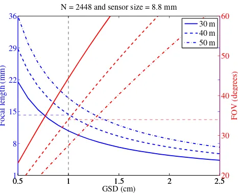
Figure 2: Focal length and Field of View (FoV) as a function of the Ground Sampling Distance (GSD) in relation to the flying height above terrain.
Camera parameters
Interface USB 2.0
Lens mount C-Mount
Sensor technology CCD
Resolution (h x v) 2448×2050
Resolution category 5 Megapixel
Color depth 8bit (14bit ADC)
Sensor size 2/3” (8.446×7.066 mm)
Shutter Global
Dimensions 34.0×32.0×34.4 mm
Mass 74.0 g
Lens parameters
Optical resolution rating 3 Megapixel
Focal length 12 mm
Back focal length 8.4 mm
Maximum aperture 1.4f
Angle of view @2/3” (h x v) 39.57°×30.14°
Optical distortion ≤0.7%
Dimensions ø30.0×51.0 mm
Weight 68.2 g
Experimental optical resolution 10−4rad≈0.34arcmin
Table 1: UEye USB UI-2280SE camera and VS Technology B-VS1214MP lens specifications
of this paper. More specifically, we have opted for a 5MP C-Mount USB camera having a 2/3” CCD-type image sensor and connected to the on-board Atom board using an USB-2.0 cable.
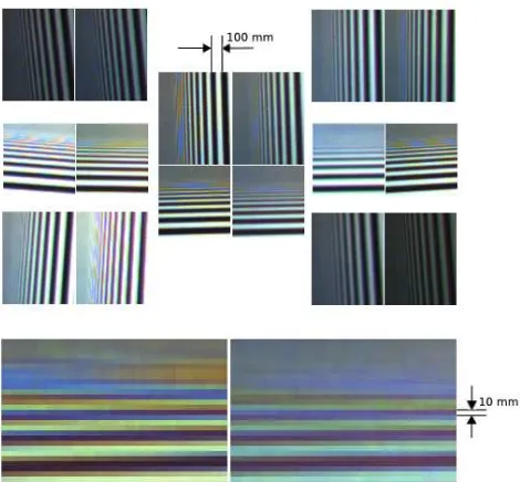
Figure 3: Resolution comparison between the 5M and the 3M lenses using the images of a resolution testing board taken from a distance of 100 m.
In order to guarantee a robust visual tracking of terrestrial targets in the presents of inevitable pitch/roll variations, as well as to maintain good geometry for mapping applications in post-processing mode (i.e. sufficient overlap and good intersections of rays), the on-board optical sensor is required to satisfy a tight trade-off between the attainable ground sample distance (GSD) and the sufficiently wide
field-of-view (FoV). The resultant correspondence between the re-quired characteristics is depicted in Fig. 2. In particular a lens hav-ing a focal length of 12 mm have been found to provide the opti-mum tradeoff between the attainable GSD and FoV.
Subsequently, a number of 12 mm lenses have been tested for at-tainable angular resolution and optical distortion. Fig. 3 portrays the resolution comparison between the 5MPixel and the 3MPixel lenses. The figure contains the full-zoom fragments from the im-ages of a resolution testing board taken from a distance of 100 m. Each pair of images contains a 3MP lens-based image on the left and a 5MP lens-based image on the right taken at the respective edge of the image frame (for instance the top-right pair of images were taken by positioning the target board at the very top-right of the visible frame). Furthermore, at the bottom of the image there is a further 5x blow-up of the 3MP and 5MP images from the center of the frame, where a single-pixel resolution may be visible. The specifications of the camera and the 3MP lens being found to satisfy the necessary requirements are summarized in Table 1. In partic-ular the camera-lens combination characterized in Table 1 exhibits an angular resolution of10−4radians. Consequently, for the sake of calculation of Eq. (20) we will assume the angular error standard deviation ofσθ= 0.0001.
4.3.1 Camera calibration procedure In order to minimize the contribution of the optical distortion errors to the overall localiza-tion accuracy, we have conducted a comprehensive calibralocaliza-tion of the optical sensor. Specifically, a free-network based camera cali-bration procedure introduced in (Luhmann et al., 2006) was carried out to estimate the essential calibration parameters using bundle adjustment. A target network was constructed in outdoor condi-tions with targets scattered in three dimensions. This is important to achieve minimum correlation between the interior and exterior ori-entation parameters, which is crucial for achieving maximum posi-tioning accuracy with the camera. Images were taken from multiple camera positions and at every location camera was rolled by 90° to ensure decorrelation of the camera perspective centre coordinates from other parameters. The targets were surveyed using a Leica TCR403 theodolite with 3mm positioning accuracy (as specified by the manufacturer).
4.4 Planar target design
Markers that are used in computer vision ([13], [9] [5], [11]).
(a) (b) (c) (d)
Figure 4: Planar marker systems utilized in computer vision (K¨ohler et al., 2010).
5 QUANTITATIVE ANALYSIS
20 30 40 50 60 70 80
0 0.05 0.1 0.15 0.2
ρ [m] σ ep
[m]
d = 1m d = 1.5m d = 2m
Figure 5: Terrestrial target horizontal position standard deviation versus MAV flight altitudeρand target sizedassuming the flight speed ofv= 5m/s and synchronization error ofτ= 1ms.
0 5 10 15 20
0 0.05 0.1 0.15 0.2
v [m/s] σ ep
[m]
τ = 1ms
τ = 3ms
τ = 5ms
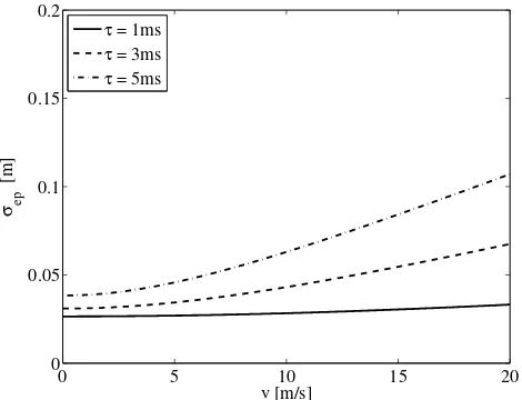
Figure 6: Target horizontal position standard deviation versus MAV horizontal speed vand sensor synchronization errorτ assuming MAV flight altitude ofρ= 40m and target size ofd= 1.5m.
Figures 5 and 6 characterize the expected standard deviation of the terrestrial target horizontal position, calculated from Eq. (20), as a function of the flight-above-terrain altitudeρand the horizontal flight speedv, respectively. In particular, Fig. 5 suggests the feasi-bility of terrestrial target localization with a precision of about 3cm from an altitude of 40m and using a target of 1.5m in diameter. Observe that the quadratic relation between the estimated position standard deviation and the flight altitude constrains the altitude at which sub-decimetre georeferencing of terrestrial targets is attain-able. Furthermore, Fig. 6 demonstrates the tolerance of the target localization accuracy to the MAV flight speed. Specifically, at the flight altitude ofρ = 40m a sub-3cm localization accuracy may be achieved with synchronization accuracy ofτ = 1msand flight speeds of up-tov= 20m/s.
6 CONCLUSIONS AND FUTURE WORK
We have carried out a simplified error propagation analysis when localizing a multi-point planar terrestrial target from a MAV plat-form in real-time. Our theoretical analysis is complemented by the quantitative characterization of the attainable performance based on specific hardware platform. Our feasibility study suggests that the cm-level (<3cm) real-time localization is attainable using com-mercially available hardware and we intend to demonstrate such functionality as part of our future research.
REFERENCES
Ascending Technologies, 2010. AscTec
Pel-ican with Autopilot User’s Manual. URL:
www.asctec.de/assets/Downloads/Manuals/AscTec-Autopilot-Manual-v10.pdf.
Fiala, M., 2010. Designing highly reliable fiducial markers. IEEE Transactions on Pattern Analysis and Machine Intelligence 32(7), pp. 1317–1324.
F¨orstner, W. and Wrobel, B., 2004. Mathematical concepts in pho-togrammetry. In: J. McGlone and E. Mikhail (eds), Manual of Photogrammetry, fifth edn, American Society of Photogrammetry and Remote Sensing, Bethesda, MA., pp. 15–180.
Javad, 2010. Javad TR-G2 Datasheet. URL:
javad.com/downloads/javadgnss/sheets/TR-G2 Datasheet.pdf.
K¨ohler, J., Pagani, A. and Stricker, D., 2010. Detection and iden-tification techniques for markers used in computer vision. In: M. Grabner and H. Grabner (eds), Visualization of Large and Un-structured Data Sets IRTG Workshop.
Luhmann, T., Robson, S., Kyle, S. and Harley, I., 2006. Close range photogrammetry: principles, techniques and applications. Whittles Publishing Dunbeath, Scotland.
Morris, W., Dryanovski, I., Bellens, S. and Bouffard, P., 2011. Robot Operating System (ROS) software stack:asctec drivers. The City College of New York. www.ros.org/wiki/asctec drivers.
Pines, D. J. and Bohorquez, F., 2006. Challenges facing future micro-air-vehicle development. Journal of Aircraft 43, pp. 290– 305.
Schwarz, K. P., Chapman, M., Cannon, M. and Gong, P., 1993. An integrated ins/gps approach to the georeferencing of remotely sensed data. Photogrammetric Engineering and Remote Sensing 59(11), pp. 1167–1674.
Schweighofer, G. and Pinz, A., 2006. Robust pose estimation from a planar target. Pattern Analysis and Machine Intelligence, IEEE Transactions on 28(12), pp. 2024–2030.
Skaloud, J. and Cramer, M., 2011. GIS Handbook. Springer, chap-ter Data Acqusition.
Wagner, D. and Schmalstieg, D., 2007. ARToolKitPlus for Pose Tracking on Mobile Devices. In: M. Grabner and H. Grabner (eds), Computer Vision Winter Workshop.