VISIBILITY ANALYSIS OF POINT CLOUD IN
CLOSE RANGE PHOTOGRAMMETRY
B. Alsadika,b,*, M. Gerkea, G. Vosselmana
a)
University of Twente, ITC Faculty, EOS department, Enschede, The Netherlands (b.s.a.alsadik, m.gerke, george vosselman)@utwente.nl
b)
University of Baghdad, College of Engineering, Surveying Department, Baghdad, Iraq
Commission V, WG V/2
KEY WORDS: visibility – point cloud – voxel – HPR – line tracing – z buffering
ABSTRACT:
The ongoing development of advanced techniques in photogrammetry, computer vision (CV), robotics and laser scanning to efficiently acquire three dimensional geometric data offer new possibilities for many applications. The output of these techniques in the digital form is often a sparse or dense point cloud describing the 3D shape of an object. Viewing these point clouds in a computerized digital environment holds a difficulty in displaying the visible points of the object from a given viewpoint rather than the hidden points. This visibility problem is a major computer graphics topic and has been solved previously by using different mathematical techniques. However, to our knowledge, there is no study of presenting the different visibility analysis methods of point clouds from a photogrammetric viewpoint. The visibility approaches, which are surface based or voxel based, and the hidden point removal (HPR) will be presented. Three different problems in close range photogrammetry are presented: camera network design, guidance with synthetic images and the gap detection in a point cloud. The latter one introduces also a new concept of gap classification. Every problem utilizes a different visibility technique to show the valuable effect of visibility analysis on the final solution.
1. INTRODUCTION
Computing the visible part of a 3D object is a vital problem in computer graphics, computer vision, robotics, GIS and photogrammetry. Usually the visibility should be accomplished in an automated way from a certain viewpoint or camera. Currently, the point clouds can be produced either by using laser scanning or dense image matching which is widely used for 3D acquisition, representation and reconstruction. These point clouds are either sparse or dense of millions points. However, a problem arises when viewing a point cloud as shown in Figure 1 where the objects looking direction cannot be identified (Katz et al., 2007). This necessitate to use the visibility testing and to discard the occluded points to properly view the object points.
Figure 1. Point cloud in an unknown looking position either forward or backward (Luigi, 2009)
The earlier digital methods of terrain visibility analysis is presented in GIS an known as viewshed analysis (Yoeli, 1985). The method is simply to analyze the Line Of Sight LOS between the observer and the target. This is by comparing the tangent of the LOS angle and the other angles of the terrain
points. The visibility is considered blocked when the tangent of the angle between the observer and an middle terrain points is greater than the tangent of the observer-to-target angle (Fisher, 1996)
.
During the last two decades, different methods were developed to solve the visibility problem in the field of computer graphics for real-time rendering and compute games (Bittner and Wonka, 2003; Cohen-Or et al., 2003). Currently, the method of hidden point removal HPR (Katz et al., 2007) is widely applied for the visibility analysis. The advantage of this technique is to avoid creating a surface from the point cloud which might be expensive and this led to analyze visibility efficiently with both sparse and dense clouds. However, when the point cloud is noisy or non-uniformly sampled, a robust HPR operator (RHPR) is preferred to be used (Mehra et al., 2010) to deal with these cases.
Other techniques are based on creating a triangulated mesh surface like by using poissons reconstruction (Kazhdan et al., 2006) or ball pivoting (Bernardini et al., 1999). After we create the surface, the notion of visibility can be uniquely defined and then find its hidden and visible points from any viewpoint. This is mathematically achieved by either intersecting the line of sight rays with the surface triangles or checking the orientation of the surface normal.
With volumetric data applications, a voxel based techniques are suitable more than triangle based. However, we cannot simply adopt those voxel techniques (Kuzu, 2004). Computing the surface normal vector is more expensive to compute and less accurate as well. Therefore line tracing and z-buffering is usually used with these volumetric data types.
In this paper, we will demonstrate the necessity of using the techniques of visibility analysis in solving three different photogrammetric problems. These visibility methods are:
The surface triangle based methods (the normal direction testing, triangle – ray intersection, Z – buffering method)
The voxel based techniques (voxel - ray intersection, ray tracing and Z- buffering method).
The hidden point removal HPR
The three different problems in close range photogrammetry addressed are: camera network design, guidance with synthetic images and the gap detection in a point cloud. While the two former examples are extracted from our previous work, the latter one introduces also a new concept of gap classification.
2. METHODOLOGY
The mathematical background of three visibility approaches will be presented in the following sections.
2.1 Surface triangulation based methods
The triangulation based methods can be applied by either testing the surface normal direction, intersection between a triangle and a line in space or by using the distance buffering by projecting the points back into a plane (image). These three methods require the creation of triangulated surface which might be expensive in terms of computations and time consuming.
2.1.1. Testing the surface normal direction: This method is considered a simple method when compared to the other two methods since it is just based on testing the angle difference between the vertex (or face) surface normal and the viewing direction. The methodology is based on creating a triangulation surface and computes the normal vector for each vertex or face. Several efficient methods are found for the surface triangulation like ball pivoting (Bernardini et al., 1999) and Poisson reconstruction (Kazhdan et al., 2006).These normal vectors are used to test the visibility of points in each camera as shown in Figure 2 which shows a simulated building facade example.
Figure 2. Visibility by using the triangular surface normal vectors
Accordingly, the decision of considering points as visible or invisible is depending on the absolute difference between the orientation of the camera optical axis � and the face normal direction . This difference is compared to a threshold (like <90o) to decide the visibility status. The algorithm pseudo code is:
� � � � � � � | |
However, it must be noted that by only using this technique, we are not able to detect and avoid occluded points. This is obvious when the angle difference is less than the threshold while the protrusion of a façade occluding the point as shown in Figure 3.
Figure 3. Incorrect visibility result
2.1.2 Ray - triangle intersection: This method and the method of ray –voxel intersection in section 2.2.1 is based on the same geometrical strategy where each triangle vertex is tested whether representing the first intersection point with the line emerging from a certain viewpoint or not. Being not the first intersection point indicates the occlusion case. Every vertex point in every camera or viewpoint should be tested to reach the final visibility labeling. This illustrates the large amount of computations needed in these geometrical intersection methods. However, it seems accurate and no incorrect visibility cases can arise. (Figure 4)
Figure 4. Visibility by testing the ray-triangle intersection
Mathematically, the intersection method is based on solving the intersection of a line and triangle in space. Möller and Trumbore (1997) developed the following efficient solution as illustrated in Figure 5.
A point on a triangle vertices ( ) is defined by
(1)
Where represent the barycentric coordinates which should fulfill the condition of � The algorithm of ray-triangle intersection is therefore to solve the following system of equations:
[
] [ ] [ ]
(2)
Where is the distance from the intersection point to the ray origin ( as shown in Figure 5.
Figure 5. Ray-triangle intersection No visibility
� �
The method is based on the geometric intersection of Line – Triangle. However, the disadvantage of this method is the difficulty of the reconstruction (surface triangulation) since it often requires additional information, such as normals and sufficiently dense input. Moreover, it is time consuming with a large data set because every triangle should be tested for the intersection. The algorithm can be summarized as follows:
� �
� � � � �
�
�
� �
| |
2.1.3 Z-buffering method: The third triangle – based technique is the Z- buffering or depth buffering method which is applied by projecting the surface triangles back to a grid plane like a digital image. These back projected 2D triangles are tested whether represent the closest or the farthest from that plane. The occluded triangles will be neglected and only keep the close triangles which should be visible from the defined viewpoint as shown in Figure 6. The final visibility map is like a digital image, but the pixel values are the ( coordinates instead of the RGB information. The pixel size should be selected carefully to avoid extra processing time or less efficient results.
Figure 6. Depth - buffering method
The algorithm can be summarized as follows:
� � � � � �
� � � �
� �
� � �
� � � �
�
� � � �
� � � �
�
� � �
2.2 Voxel based approach
In some applications like gaming or other computer graphics applications, the point cloud is represented as voxels and it seems very useful to analyze the visibility on the basis of voxels rather than points. The advantages of using these methods are the avoidance of creating a surface while it is considered an expensive approach in terms of computer memory. Three different techniques are listed in the following sections which are: voxel –ray intersection, voxel distance buffering and ray tracing methods.
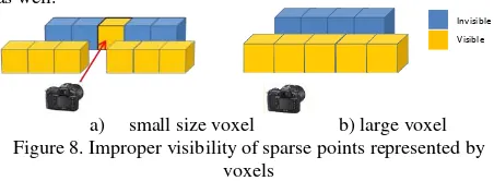
2.2.1.Voxel – ray intersection: In this technique, the visibility test is applied by intersecting a ray emerging from the viewpoint (origin-o) with a certain direction to the voxels ( ) and to check if it intersects (flag=1) or not (flag=0) as shown in Figure 7. This is a typical line-box intersection problem presented by Williams et al. (2005) and coded by Mena-Chalco (2010). Turning the point cloud into voxels is simply driven by gridding the space occupied by the points according to a specific voxel size. This is followed by discarding the empty voxels and keeping all the occupied voxels as shown in Figure 7.
Figure 7. Voxel-ray intersection for visibility
To speed up the computations of the intersection algorithm, a bounding volume hierarchy BV is created (Smits, 1998). Mathematically, the intersection involves computing the distance from the origin to the intersection point which object was hit Mena-Chalco (2010).
The advantages of this method beside the avoidance of surface reconstruction are that no settings are required to implement the method except the voxel size to get better accurate results. However, disadvantages of this method arise when processing a large data set because it may be expensive in terms of time and memory consumption. Furthermore, a sparse point cloud will not be modeled efficiently since empty space between voxels can produce wrongly visible points (Figure 8a). Although, enlarging the voxel size (Figure 8b) might avoid this problem but probably mislead the visibility results in some applications as well.
a) small size voxel b) large voxel Figure 8. Improper visibility of sparse points represented by
voxels
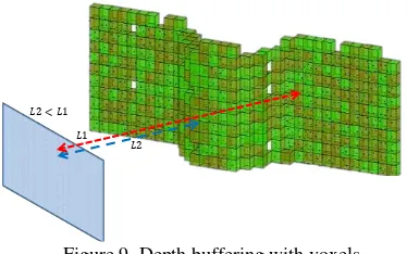
2.2.2 Buffering technique: The distance buffering method is applied in a same way as in the triangle buffering method. Projecting the voxels back to a grid plane and testing whether the 2D polygons represent the closest or the farthest from that plane. The occluded polygons will be neglected and only keep the closest which should be visible from the defined viewpoint as shown in Figure 9. The time consuming is a main disadvantage of this method.
Origin
�
Invisible
Figure 9. Depth buffering with voxels
2.2.3 Ray tracing technique: The ray tracing method or voxel traversing is simply implemented by computing tracing points (or voxels) along the ray toward the destination voxel. These tracing points will be computed at every small interval which is less than the voxel size. Then it is tested whether they intersect or hit a voxel before reaching the destination. The voxels will be labeled as visible or hidden based on this methodology as shown in Figure 10.
Figure 10. Line tracing with voxels
It is worth to mention that the difference between the ray tracing method and the methods of buffering and ray–voxel intersection is mathematically:
- The ray tracing method is a forward computations starting from the viewpoint position and proceed in specific intervals. - The ray-voxel intersection is an inverse computations between the voxels in question and the viewpoint.
2.3 Hidden point removal (HPR)
The concept of this method (Katz et al., 2007) is to extract the points that are located on the convex hull of a transformed point cloud obtained by projecting the original point cloud to a dual domain to find the visible points.
The method is developed to process the data in two steps: inversion and convex hull construction.
The “spherical flipping” is used to reflect every point pito a
bounding open sphere along the ray connecting the viewpoint and pi to its image outside the sphere. The convex hull construction is followed by using the set that contains the transformed point cloud and the viewpoint. The major advantages of this method are to determine the visibility without reconstructing a surface like in the previous surfacing methods beside the simplicity and short time implementation (Figure 11). Moreover, it can calculate visibility for dense as well as sparse point clouds, for which reconstruction or other methods, might be failing. However, the disadvantage is realized when a noisy point cloud exists (Mehra et al., 2010). Moreover, it is necessary to set a suitable radius parameter that defines the reflecting sphere as will be shown in the experiment.
Katz et al. (2007) suggested to solve the problem of finding the proper radius R automatically by adding additional viewpoint, opposite to the current viewpoint. Then analyzing the visible points from both viewpoints and minimizing the common points by optimization minimization technique like the direct
search method. This is based on the fact that no point should be visible simultaneously to both viewpoints
Figure 11. HPR method (Katz et al., 2007)
A Matlab code is written to find out the radius value as follows which is inspired from the general code of the authors.
optimR=@(x)estimateR(x,p,C1,C2);% C1,C2 are the viewpoints, p:points,x:parameter.
[x,fval] = fminsearch(optimR,x0)
function [f,rr]=estimateR(x,p,C1,C2)
dim=size(p,2); numPts=size(p,1);
p1=p-repmat(C1,[numPts 1]);%
normp1=sqrt(dot(p1,p1,2));%Calculate ||p|| R1=repmat(max(normp1)*(10^x),[numPts 1]); rr= log10(R1);%%Sphere radius
P1=p1+2*repmat(R1-normp1,[1
dim]).*p1./repmat(normp1,[1 dim]);%Spherical flipping
visiblePtInds1=unique(convhulln([P1;zeros(1,dim)]));%co nvex hull
visiblePtInds1(visiblePtInds1==numPts+1)=[]; P1=p(visiblePtInds1,:);
p2=p-repmat(C2,[numPts 1]);%
normp2=sqrt(dot(p2,p2,2));%Calculate ||p||
R2=repmat(max(normp2)*(10^x),[numPts 1]);%Sphere radius
P2=p2+2*repmat(R2-normp2,[1
dim]).*p2./repmat(normp2,[1 dim]);%Spherical flipping
visiblePtInds2=unique(convhulln([P2;zeros(1,dim)]));%co nvex hull
visiblePtInds2(visiblePtInds2==numPts+1)=[]; P2=p(visiblePtInds2,:);
A = setdiff(P1,P2,'rows'); f= -mean(sum(abs(A))
3. Applications in close range photogrammetry
To show the importance of the aforementioned visibility testing methods, we will present three different problems in close range photogrammetry. The problems are: the camera network design, the creation of synthetic images for guiding the image capture and the gap detection in a dense point cloud.
The first two applications of the camera network design and guiding the image capture were introduced previously in (Alsadik et al., 2013). The concept was to build an automated imaging system for the 3D modeling of cultural heritage documentation. The system was mainly designed to assist non-professionals to capture the necessary images for having a complete and reliable 3D model. This image capturing was based on creating synthetic images from the same viewpoints that is designed in the camera network. However, in this paper we will emphasize on the role of the visibility analysis to have sufficient results.
Moreover, a method of detecting gaps in the dense points cloud will be presented where a voxel based visibility analysis will be a crucial factor to reach sufficient results. The actual challenge is to differentiate between openings in the object and gaps caused e.g. by occlusion. These three applications will be explained and a solution will be presented in the following sections with the impact of the visibility analysis on the solution for each problem.
3.1 Camera network design
A basic necessary step in any photogrammetric project is to carefully design the camera network. This design needs a high expertise and a thorough planning. Different elements are to be modeled like the Base/Depth ratio, the uncertainty in image observation and the ground sample distance GSD. Furthermore, the visibility of object points from the different camera locations is an important factor during the design of the imaging network. In other words, we should carefully compute for every part of the object of interest, the imaging cameras according to their designed orientation. Any of the aforementioned methods of visibility can be used to test the visible points like by testing the vertex normal directions of Figure 12(a). A rough point cloud of the object is first acquired from a video image sequence and then a triangulation surface is to be created (Alsadik et al., 2013). This created rough model is necessary to design a sufficient camera network that almost ensure a high amount of coverage and accuracy. The design is to be arranged in a way that ensures points to be viewed by at least three cameras (Luhmann T. et al., 2006) for a high positioning reliability.
In order to find the minimal efficient camera network, a dense imaging network is firstly to be simulated. This dense network is then filtered on the basis of removing redundant cameras in terms of coverage efficiency and the impact on the total accuracy in the object space. Accordingly, the filtering is based on evaluating the total error in the object space and computing the effect of each camera on this error. The least effective redundant camera in terms of accuracy will be neglected. The whole procedure of filtering will be iterated until reaching the desired accuracy (by error propagation) or when no more redundant cameras are exist in the imaging network.
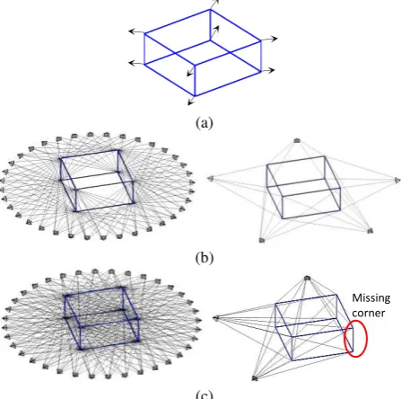
The simulation test of Figure 12 shows a rectangular building surrounded by 36 cameras with the imaging rays. However, this dense network can be reduced to a minimal network by filtering the redundant cameras basing on the total object points accuracy. To apply the filtering correctly, a visibility testing is needed. The direction of the vertices normal is used to decide if point is visible in camera and so on as discussed in section 2.1.1.
(a)
(b)
(c)
Figure 12. (a) vertex normal orientation. (b) Dense and minimal camera network with visibility test. (c) Dense and minimal network without visibility test.
The minimal camera network with visibility testing is shown in Figure 12b where only five cameras are needed to have a sufficient coverage and accuracy for the object measurements by photogrammetric techniques. However, the same network wrongly reduced into only three cameras as shown in Figure 12c where no visibility is considered and all the points are assumed visible in all the viewing cameras. This results in a wrongly designed network despite the preservation of three viewing cameras per point where one of the corners will actually missed as shown in the red circle of Figure 12c.
3.2 Synthesizing images
In some applications of photogrammetry and CV a guidance is needed to have a correct captured images like for 3D modeling and panoramic imaging. The motive to create the synthetic images is the suitability of these images to guide the camera operator, even non-professionals, to the desired optimal location and camera attitude. We proposed previously a simple way to guide the camera operator to capture high-resolution HR images for 3D modeling. The key idea is to create, based on the designed camera network, multiple synthetic images of the object to be modeled. This is followed by an image matching to decide the amount of equivalence or similarity between the real captured images and the synthetic images (Alsadik et al., 2013).
Therefore, even if the image matching might be insufficient in some cases, the camera operator can visually inspect and capture the desired image. Moreover, these synthetic images and then guidance are suitable to be applied by smart phones and autonomous navigation robots as well. The synthetic images are formed by first, create a 3D triangulated surface from initial point cloud by any efficient surfacing techniques like ball pivoting (Bernardini et al., 1999) or Poisson reconstruction (Kazhdan et al., 2006). Accordingly, image resampling is implemented to get a textured 3D cloud or model. A free web application software like 123D catch (Autodesk, 2012) or a combination of open source software like VSfM (Wu, 2012), SURE (Wenzel, 2013) and Meshlab (Meshlab, 2010) can also be used to create such a textured low detailed model.(Figure 13). This textured 3D model will be transformed by collinearity equations to the designed viewpoint (see previous subsection) to create the synthetic images.
(a) (b) (c)
(d)
Figure 13. (a) Rough point cloud. (b) Surface mesh. (c) Textured mesh. (d) Synthesizing images Missing
The information about the textured 3D model is simply transformed in two steps back to the intended synthetic images. The first is to project the 3D coordinates back into the 2D pixel coordinates and the second is to assign the texture for each triangular face. Therefore, each textured triangular face (three vertices and the patch RGB color) is transformed as illustrated in Figure 13 from the texture image to the corresponding synthetic image by linear interpolation. The transformation is done for each face by moving across a bounding rectangle and assigning the pixel value from the texture image to each pixel falls inside the triangle.
Figure 14 shows a sample of the synthetic images of a fountain in the first row and their equivalent real images in the second row.
Figure 14. Synthetic and real captured images.
The synthesizing approach should account for the visibility condition otherwise a wrong texture can deteriorate the created synthetic image. Figure 15 shows the effect of self-occlusions if the visibility is not considered. The z-buffering technique of visibility is applied and based on testing if the same pixel in the synthetic image is covered more than one time. Accordingly, the pixels representing further points are excluded while keeping the closest pixels.
Figure 15. Self-occlusion in synthetic image with and without visibility test
3.3 Gap detection in a point cloud
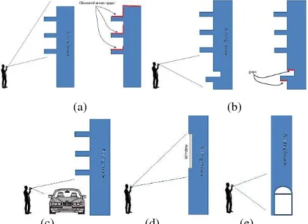
The gap identification in the image based point cloud of architectural structures is a challenging task. The challenge is in the sense of automation and the difficulty to discriminate between true gaps (openings) and gaps in a point cloud caused by occlusion. Figure 16 summarizes some possible causes of gaps that might be found in the image based point cloud. These gaps can be:
Obscured parts because of perspective, e.g. roof parts are not visible because of self-occlusion when viewed from a street level (a).
Occluded parts of the object like the protrusion in facades or vehicles near facades (b, c).
Texture-less parts of the object like white painted walls and window glass (d).
Openings like corridors and open gates of a building (e).
However, it seems that different techniques can be followed to identify these gaps. The detection of gaps in 3D is to be accomplished either by using a volumetric representation with voxels or with triangulated surface meshing. With voxels, the
well-known robotics technique of “occupancy grid” can be used to decide which voxel is occupied and which one is empty (Thrun et al., 2005). However, this is usually implemented with a moving robot and where there is uncertainty in the voxel labeling. In surface triangulation methods, the gap may be detected by looking for the skewed elongated triangles which is an indication for the gap existence (Impoco et al., 2004).
(c) (d) (e)
Figure 16. Gaps cause. (a) Obscured parts from street view. (b) Protrusions in facades. (c) Occlusion effect. (d) Texture-less parts. (e) Real openings.
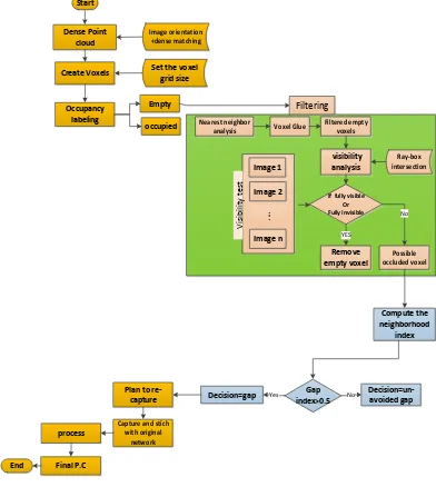
In this paper, the gap detection is solved by the following technique which is based on volumetric space representation, followed by a classification into gap or opening:
The space occupied by the point cloud is to be filled with voxels and each voxel is labeled as empty or occupied based on the points existence within that voxel. The empty voxels are to be investigated for the gap detection. However, these detected gaps might be openings or gaps because of occlusions as mentioned before. In this sense the methodology of detection is summarized as:
- Construct the voxels in 3D space and preferably with octree to save memory and processing time. Label each voxel as empty or occupied.
- Preliminary filtering to account for noise in the point cloud.
- Test the visibility with the line tracing or voxel-ray intersection method.
- Filter empty voxels after classifying the remaining voxels based on visibility into fully occluded, partially occluded, and fully visible.
- Compute the neighborhood index (NI) to assist the decision of labeling occluded voxels.
- Classify the occluded voxels into either openings or gaps.
The first step of filtering the blundered empty voxels is based
on what we call “voxel glue”. This is computed by using the
occupied voxels to glue the neighboring empty voxels and discard the others. This is to be done by searching for the
nearest empty voxels by using the ‘nearest neighbor’ technique.
This is followed by removing the non-glue empty voxels which represent the marginal or bordering voxels away from the occupied voxels of the point cloud. Then a second step of filtering is based on the visibility analysis from the designed viewpoints as discussed in section 2.2. Three cases might be found as illustrated in Figure 17: fully occluded, partially occluded, and fully visible voxels.
Fully visible and fully occluded empty voxels will be neglected while partly occluded voxels will be more investigated as potential gaps or openings. Neglecting fully visible voxels is
based on the fact that empty voxel cannot occlude occupied voxels (Figure 17b). On the other hand fully hidden voxels like empty space behind a wall are also neglected as illustrated in Figure 17a.
(a) (b) (c)
Figure 17. Empty voxels and visibility analysis. (a) Fully occluded. (b) Fully visible. (c) Partly occluded.
However, such a visibility index is not sufficient to reliably find out the potential gaps. This is because of the possible inadequate camera placement and the blunders or noise in the point cloud.
Therefore, other measures are to be added. A neighborhood index (NI) might be efficient to strengthen the detection of empty voxels, this is actually similar to a majority filter (3x3x3 neighborhood), but also uses the actual direction of neighbors. Figure 18 illustrates the computation of the neighborhood index of a voxel. Three types of proximity distances ( ) are computed to define the search space. More neighboring occupied voxels indicate a high chance of being an occluded empty voxel and vice versa. NI is computed as (number of empty voxels/ total neighboring voxels) and a threshold of (>50%) is considered to indicate a blundered empty voxel.
(a)
(b)
Figure 18. (a) Proximity measure. (b) 3*3 neighboring voxels
The measure of the altitude can be used. Altitude index is useful when the imaging is done with a street level view since the upper parts of the object are self-occluded. Hence, the empty voxels near the upper parts of objects are labeled as occluded gaps. Finally, a discrimination between the openings and occluded gaps is needed. Therefore, openings can mislead information and then to define openings.
After the gap detection, auxiliary images are to be captured to
Figure 20 illustrates the workflow of the proposed gap detection method in image based point clouds and the impact of visibility analysis.
Figure 20. The methodology of gap detection
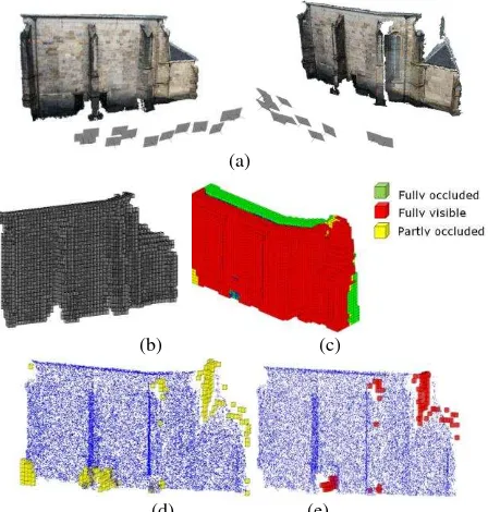
An experimental test of a gap detection is illustrated in Figure 21 where a building facade with extruded columns is to be modeled with images. Thirteen images are taken to the facade and a dense point cloud is acquired after image dense matching (Figure 21a). Obviously, the façade point cloud includes only gaps caused by occlusions and the insufficient camera network coverage. The point cloud is voxelized and then the voxels are labeled either empty voxels or occupied voxels as shown in Figure 21b. The visibility analysis by using the ray-voxel intersection is applied as shown in Figure 21c. The presented filtering strategy based on the visibility, neighborhood index and altitude resulted in the final empty voxels which represent the occluded gaps in the point cloud. Figure 21d shows the empty voxels according to their visibility status from the cameras. Figure 21e shows the final result of gap detection.
(a)
(b) (c)
(d) (e)
Figure 21. Gap detection with voxels. (a) The dense point cloud. (b) The occupied voxels. (c) The empty voxels and visibility analysis. (d) The detected empty voxels after visibility analysis. (e) Final occluded gaps after neighborhood analysis.
4. CONCLUSION AND DISCUSSION
In this study, three strategies are described to analyze the visibility of 3D point clouds and these are (surface based, voxel based, and HPR). Every method has its advantages and disadvantages in the sense of accuracy, time consuming, a priori settings and efficiency of the results. Accordingly, the use of visibility analysis is quite important in many photogrammetric applications and especially when the data set type is a point cloud.
Three problems were selected in close range photogrammetry where the visibility plays a vital role to have a successful result. Every visibility solution to the three problems was applied by using one of the techniques presented in section 2.
Visibility analysis in the first application of camera network design was crucial to have a sufficient overage as shown in Figure 12. The vertex normal orientation testing is used in this case for simplicity since the object is represented by only eight corner points.
The second experiment showed the effect of visibility analysis on creating synthetic images of a 3D model. Figure 15 showed the effect of self-occluded parts of the final synthetic images if the visibility analysis is neglected. The technique of z-buffering with triangular surfaces proved its efficiency and suitability to deal with such kind of surface mesh data.
The third test presented the problem of gap detection in a point cloud produced from images. The space is modeled as volumetric voxels. Hence, the proposed solution is based mainly on testing the visibility of voxel-line intersection method of section 2.2.1. This visibility is also supported by other measures like neighborhood index and altitude information.
Future work can investigate for other visibility techniques which can handle for both sparse and dense point cloud data and investigate which of the current methods is the most efficient for handling the photogrammetric application.
5. REFERENCES
Alsadik, B., Gerke, M., Vosselman, G., 2013. Automated camera network design for 3D modeling of cultural heritage objects. Journal of Cultural Heritage 14, 515-526.
Autodesk, 2012. 123D Catch http://www.123dapp.com/catch. Autodesk.
Bernardini, F., Mittleman, J., Rushmeier, H., Silva, u., Taubin, G., 1999. The Ball-Pivoting Algorithm for Surface Reconstruction. IEEE Transactions on Visualization and Computer Graphics 5, 349-359.
Bittner, J., Wonka, P., 2003. Visibility in computer graphics. Environment and Planning B: Planning and Design 30, 729-755.
Cohen-Or, D., Chrysanthou, Y.L., Silva, C.T., Durand, F., 2003. A survey of visibility for walkthrough applications. IEEE Transactions on Visualization and Computer Graphics 9, 412-431.
Fisher, P.F., 1996. Extending the Applicability of Viewsheds in Landscape Planning Photogrammetric Engineering and Remote Sensing (PE&RS) 62, 1297-1302.
Impoco, G., Cignoni, P., Scopigno, R., 2004. Closing gaps by clustering unseen directions, Shape Modeling Applications, 2004. Proceedings, pp. 307-316.
Joy, K.I., 1999. The Depth-Buffer Visible Surface Algorithm, Computer Science Department, University of California. , pp. 1-5.
Katz, S., Tal, A., Basri, R., 2007. Direct Visibility of Point Sets. ACM Transactions on Graphics 26.
Kazhdan, M., Bolitho, M., Hoppe, H., 2006. Poisson surface reconstruction, Proceedings of the fourth Eurographics symposium on Geometry processing. Eurographics Association, Cagliari, Sardinia, Italy, pp. 61-70.
Kuzu, Y., 2004. Volumetric Object Reconstruction by Means of Photogrammetry, Civil Engineering and Applied Geosciences. Technical University of Berlin p. 151.
Luhmann T., Robson S., Kyle S., Hartley I., 2006. Close Range Photogrammetry Principles, Methods and Applications. Whittles Publishing Country, United Kingdom.
Luigi, A.G., 2009. MyCrustOpen. , File Exchange - Matlab. Mehra, R., Tripathi, P., Sheffer, A., Mitra, N.J., 2010. Technical Section: Visibility of noisy point cloud data. Comput. Graph. 34, 219-230.
Mena-Chalco, J.P., 2010. Ray/box Intersection. MathWorks Inc. Massachusetts, U.S.A., Matlab file exchange.
Meshlab, 2010. Visual Computing Lab - ISTI - CNR. http://meshlab.sourceforge.net/.
Möller, T., Trumbore, B., 1997. Fast, Minimum Storage Ray/Triangle Intersection. Journal of Graphics, gpu & game tools 2, 21-28.
Smits, B., 1998. Efficiency Issues for Ray Tracing. Journal of graphics tools 3, 1-14.
Thrun, S., Burgard, W., Fox, D., 2005. Probabilistic Robotics (Intelligent Robotics and Autonomous Agents). The MIT Press.
Wenzel, M.R.K., 2013. SURE - Photogrammetric Surface Reconstruction from Imagery, in: http://www.ifp.uni-stuttgart.de/publications/software/sure/index.en.html (Ed.).
Williams, A., Barrus, S., Morley, R.K., Shirley, P., 2005. An efficient and robust ray-box intersection algorithm. Journal of Graphics, GPU, & Game Tools 10, 45-60.
Wu, C., 2012. Visual SFM: A Visual Structure from Motion System, University of Washington in Seattle.