USER-ASSISTED OBJECT DETECTION BY SEGMENT BASED SIMILARITY
MEASURES IN MOBILE LASER SCANNER DATA
S. Oude Elberink*, B. Kemboi
Faculty of Geo-Information Science and Earth Observation, University of Twente, Netherlands - [email protected], [email protected]
Commission III, WG III/2
KEY WORDS: Segmentation, Object Detection, Semi-Automatic, Mobile Mapping Systems, Segment based Classification
ABSTRACT:
This paper describes a method that aims to find all instances of a certain object in Mobile Laser Scanner (MLS) data. In a user-assisted approach, a sample segment of an object is selected, and all similar objects are to be found. By selecting samples from multiple classes, a classification can be performed. Key assumption in this approach is that a one-to-one relationship exists between segments and objects. In this paper the focus is twofold: (1) to explain how to get proper segments, and (2) to describe how to find similar objects. Point attributes that help separating neighbouring objects are presented. These point attributes are used in an attributed connected component algorithm where segments are grown, based on proximity and attribute values. Per component, a feature vector is proposed that consists of two parts. The first is a height histogram, containing information on the height distribution of points within a component. The second contains size and shape information, based on the components’ bounding box. A simple correlation function is used to find similarities between samples, as selected by a user, and other components. Our approach is tested on a MLS dataset, containing over 300 objects in 13 classes. Detection accuracies heavily depend on the success of the segmentation, and the number of selected samples in combination with the variety of object types in the scene.
1. INTRODUCTION
The number of Mobile Mapping Systems (MMS) is increasing rapidly over the past few years. Applications can be found in fields related to urban safety analyses and/or asset management. Many MMS systems carry video cameras and laser scanner systems. Mobile laser scanner (MLS) data is a very rich data source for making inventories of the condition and number of objects in an urban environment. The huge amount of 3D points contain information on size, shape and location of objects, and their in-between distances.
The problem is to accurately find these objects in a dataset that also includes the surrounding area with many other complex shaped objects. Existing methods to classify MLS data can be divided into rule based approaches where the rules describe how the objects of interest look like, and training based methods. We present a method that aims for finding all instances of an object selected by an operator. Our approach is based on the knowledge that objects which are similar in reality will have similar appearances in point cloud data, and on the assumption that an operator is very well capable of recognizing one instance of the object(s) of interest in the data.
The motivation for this approach is that a data sample of a certain object is a good initial guess of how other instances of that object appear in the data, as it implicitly holds information on scanner configuration and point density. This enables the possibility to use this algorithm for different kinds of objects and even different kinds of point clouds, e.g. indoor and outdoor, mobile and terrestrial laser data.
The challenge in this approach is to segment the data into meaningful components, and to propose reliable similarity
measures that can handle noisy data. Our first contribution to the field is proposing a novel procedure to segment urban objects in MLS data. The second contribution is presenting a generic workflow that can deal with many different types of objects, making use of the scene knowledge of an operator. In section 3 a segmentation algorithm is presented that aims for minimizing segmentation errors in MLS data. Section 4 explains which features are calculated to the segments, and how these are used to detect objects and to classify the data. In section 5 results are given and explained to emphasize the strengths and limitations of our approach, followed by an outlook in section 6. Conclusions are given in section 7. In this paper the terms components and segments are used alternately; these terms have the same meaning in this paper.
2. RELATED WORK
Vosselman (2013) describes a two stage segmentation step in order to get meaningful segments in ALS data. In the first stage large planar segments are detected; in the second stage points from the remaining small segments are further grouped in an modified connected component algorithm, or in that paper called a segment growing algorithm, taking into account the local normal direction scaled by the local planarity.
Rules can be incorporates in point based methods and segment based (Pu et al, 2011). The success of detecting of pole like objects, as described by Brenner (2009), Lethomäki et al (2010), show that urban objects often can be found by defining a good set of rules, which are useful to translate real object shapes to how they appear in the data. Rules are often derived by researchers by processing and testing a limited amount of datasets. Main limitation of rule based classifiers is that if the dataset is different, e.g. in point density or scanning The International Archives of the Photogrammetry, Remote Sensing and Spatial Information Sciences, Volume XL-3, 2014
configuration, or if user is interested in other objects, the rules should be adapted. The problem is that the rules are often hidden in the classification algorithms, and not easy to change for an operator other than the developer. Training based classification methods as proposed by Golovinski et al, (2009) and Velizhev et al (2012), are more flexible in the sense that an operator can train the classifier depending on the objects in the scene.
Golovinskiy et al (2009) presents a min-cut algorithm on point clouds to separate foreground objects from the background. They show that using a fixed radius in connected component analysis causes under and over segmentation. Their solution to use min-cut is based on neighbourhood relations and a radius that defines the distance between the object of interest and background points. An automatic determination of the optimal radius per object to cut the graph performs better than a fixed radius.
Velizhev et al (2012) use key point feature extractors to detect object in MLS data, introducing and adapting spin images to point cloud processing. Main limitation in that approach is that the success rate depends on how well the center point of an object can be found.
Lai and Fox (2010) describe how to detect urban and indoor objects using information from objects from Google’s 3D Warehouse. They deal with segmentation errors by using a collection of different segmentation results, a so-called soup of segments, as proposed earlier by Malisiewicz and Efros (2007). This works well if enough training data is available to correctly interpreted the variety of segment collections, and if the training data correspond to the situation the dataset. Their segmentation results depend on a proper choice of a fixed threshold to define a voxel size.
The combination of using proximity and point attribute values as explained by Vosselman (2013) is what is adopted for segmenting MLS data in this paper. Next, the aim is to design a more generic approach than described by Velizhev et al (2012) to detect objects in an urban scene.
3. SEGMENTING MLS DATA INTO SINGLE OBJECTS
3.1 Design of segmentation algorithm in MLS data
The objects of interest in MLS data varies from street furniture, building facades, cars, curb stones, vegetation, rail road infrastructure. When examining the objects in a (rail) road environment, one can conclude that there are no objects of interest that only consist of a single planar surface. The ground and facades are no planar objects, considering the details such as curb stones, gardens, subtle depth variations at a building facade. Only parts of object are planar, such as doors, windows, some individual walls and locally planar road patches. A traffic sign as such is often planar, but is often attached to a non-planar object like a cylindrical pole. Thus, a planar segmentation algorithm will result in over-segmentation and will not be sufficient to group points from an object of interest into a segment. Various authors therefor describe methods to remove the ground, and perform a connect component analysis on the above ground objects (Pu et al, 2011; Lethomaki et al, 2010). A connected component analysis has the advantage that it groups points that are close together, independent of the local shape of the object. The disadvantage is that it can group points together of different objects when these are close to each other, resulting in an under segmentation of the dataset. Situations like this can be seen when wires, e.g. power lines, connect two or more objects, e.g. portals, together. If there are sufficient laser points reflected from the wire, this may cause that the wire and the two objects are considered to be one component. Also, neighbouring
trees which branches touch, are likely to be detected as one component. Our design is such that it aims for a one-to-one relation between component and object. For this several point attributes are introduced that act as constraints during the connected component algorithm, next to proximity of points. In 3.2 point attributes are presented, followed by a description how the attributes are used in forming components. In 3.4 the focus is on how get components from individual trees, even if they are close together.
3.2 Point feature calculation for seed growing algorithm
For all points three types of point attributes are calculated, based on nearby other points. These point attributes will be used later as constraints in the connected component analyses.
3.2.1 Relative height in fixed radius
For each point, the relative height is calculated in relation to the lowest point within a certain 2D radius, e.g. 50 cm. The relative height attribute is used in the attributed connected component growing algorithm to detect the ground segments.
3.2.2 Eigen vectors and normal directions for linearity and planarity
Linear features such as wires are an important cause of under-segmentation of the dataset, as it connects at least two objects attached to the wire. The linearity is calculated to use this as a feature in the attributed connected component algorithm to separate linear features from others. Linearity is calculated by Eigen vector analyses, as proposed in Bremer et al (2013).
3.2.3 Loneliness of a point
This is a density measure that measures how many points are in certain sphere around the point. Additional it counts whether these nearby points are from the same sensor or not. Most of the Mobile Mapping Systems are equipped with two laser sensors that capture the scene from another perspective. There is a few seconds of time difference between recording from one sensor to the other. Dynamic objects are therefore captured at different locations by the two sensors. These measures are used for detecting lonely points, and points on dynamic objects such as cars and pedestrians. The lonely points are considered as noisy point that may cause segmentation errors later in the process.
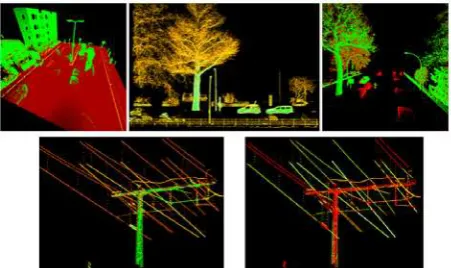
Figure 1 Point feature attributes: height above ground (top left), loneliness (top middle and bottom left), percentage of points
from other sensor (top right) and linearity (bottom right).
3.3 Attributed connected components to get above ground objects
The first connected component algorithm aims to detect ground points in MLS data. Here, the relative height is used as attribute constraint, connecting all nearby points within a certain The International Archives of the Photogrammetry, Remote Sensing and Spatial Information Sciences, Volume XL-3, 2014
neighbourhood and relative height difference of, for example, maximum 15 cm. The components with points with relative height between 0 and 15 cm are considered as ground components and removed from the dataset.
The remaining points are input for the second connected component calculation that aims for segmenting all above ground objects.
Each above ground component is established by connecting a selection of nearest neighbours that fulfil criteria on point attributes. The selection of nearest neighbours is based on the ‘k’, i.e. the maximum number of neighbours and the radius. This means that if the density is high, the selection is bounded by the maximum number of nearest neighbours. If the density is low, the growing radius will bound the selection of points. This is important to know, when trying to minimize the over- and under-segmentation on objects of interest in a certain dataset with specific scanning configuration. The number of neighbours and the radius should be chosen such that it connects points of two neighbouring scan lines.
The attribute features used as constraint during the segment growing is the linearity and the loneliness of points. For this a threshold is set to separate linear points from others. The threshold is set close to 1, in order to only separate the really linear objects such as wires. Components with a majority of points with a low number of nearby points and high linearity, e.g. at the wires, are separated from the other points. For these remaining points, a connected component algorithm is performed without attribute constraints to avoid over-segmentation on nonlinear objects, see figure 2. Of course, there may be rule based classifiers that are more specific in detecting rail road wires such as Oude Elberink et al (2013) and Beger et al (2011). We only show a rail road dataset here to show that linearity and local density can be used to cut an component into more meaningful segments.
Figure 2 Typical connected component only based on proximity (left), removal of linear components (middle, red) to
remove points on wires (right).
3.4 Identifying individual trees in a component
Typically, in a connected component segmentation groups of trees are connected into one segment when their branches are within growing radius distance. Physically, neighbouring trees may be separable, however in a point cloud it becomes rather arbitrary to assign points to an individual tree when the point density is equal or lower than the distance between branches of different trees. Still, our aim is to segment the individual trees as good as possible. The knowledge that is used is that at breast height neighbouring trees normally do not touch each other. For every segment points are selected in the range between 0.5 and 1.5 meter above the ground. For those points it is checked whether they form one or multiple components. In the latter case, we perform a growing algorithm starting at these seeds at a height between 0.5 and 1.5 m.
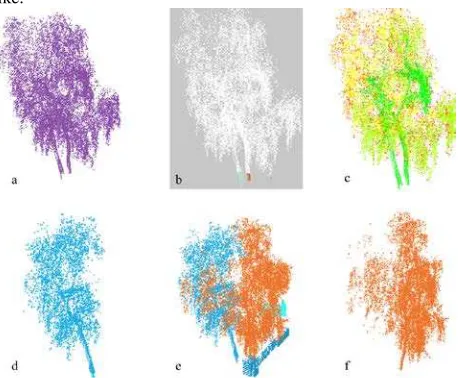
The working is as follows. For every point in the original component we built-up a capacious kd-tree with k-nearest neighbours within a certain radius, for example maximum 100 neighbours in a maximum radius of 1.5 meter. However, at this earliest stage we do not use all these neighbours for growing the segment. In order to avoid growing too rigorously, we start with using points within a small growing radius of slightly larger than the point spacing at that seed location. In an iterative growing algorithm the growing radius increases stepwise. By doing so, the structure of the tree is naturally followed as point densities in MLS data are higher at the lower part of the tree. The point density gradually decreases when approaching the tree top and the outer ends of the branches, so for these outer points a larger growing distance is required. The consequence of this method is that every point is assigned to the component that has the minimum longest distance on the route between that point and the seed. If in a single iteration a point can grow into more than one component, the distance to the nearest seed of all components is leading. In figure 3 a situation is shown where two trees are close together, and their branches are entwined. Figure 3c is coloured by the iteration number starting at 1 (green) to 8 (orange). In every iteration 5 cm is added to the growing radius, so the points at the outer ends of the trees need a growing radius of 40 cm more than at the bottom of the tree. The initial growing radius was 5 cm; eventually all points of the original component were reached with 45 cm growing radius in the 8th iteration. Figure 3e shows how the final components look like.
Figure 3 Original tree component (a), two seeds found at lower part of stems (b), points coloured by iteration number while
growing (c), (d) and (f) are final individual components visualized separately and together in (e).
If during the first iteration all points can be grown from one seed to the other, the result will be grouped into one component. This corrects an needless split of a segment, e.g. at building facades where windows may cause a split when only looking at points in between knee and breast height.
3.5 Tagging components from moving objects
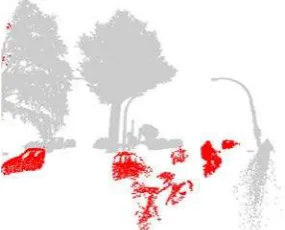
After the connected component analyses, it is directly known how many points are from one and the other sensor. This gives information on the likeliness that the object moved during the acquisition. A component is flagged as dynamic object if more than 90% of the points only has k-neighbours from the same scanner, see figure 4. Information on whether the object moved or not is useful in case of removing these objects, or selecting The International Archives of the Photogrammetry, Remote Sensing and Spatial Information Sciences, Volume XL-3, 2014
appropriate samples for these moving objects. After all, a moving car may have other shape properties than a static one.
Figure 4 Dynamic objects (red) detected by using knowledge of a two sensor system.
The heights of all above ground components are related to the nearest points in the ground components. This enables us to produce components with a height relative to the ground.
4. SEGMENT BASED SIMILARITY MEASURES
4.1 Methodology overview
In the previous section a method for getting components of above ground objects has been explained. In this section we will describe how to detect similar components and how to classify the components. In the beginning of this phase, the user is incorporated for the first interpretation of the components. In a labelling stage the user selects a component and gives a certain label to the component. The user can choose to produce one training sample if the task is to find all instances from this one sample, or the user can produce multiple samples from multiple classes if the task is to classify the data. In the remainder of this paper, the components selected by the user are called samples or sample components.
4.2 User assisted sampling
Our starting point is that the user knows what kind of objects to find in the data. How many types of traffic lights, lamp posts and traffic signs are in the scene? Are there bus shelters in the scene, and do they all look similar? This information is very helpful in selecting sample components. The selection consist of giving a class label to a component. The number of classes varies per application and per area, so the user is free to add classes if necessary.
4.3 Height histograms
Height histograms are produced by counting how many points are in a component at different height levels, called bins. Height histograms contain information on the relative distribution of points per object, and are taken as signature for describing the shape of the object. Each bin is considered as one feature in the feature vector, and each bin count is the corresponding feature value. The motivation for using height histograms is that many of our objects of interest have a typical structure when looking along the z-axis. As in the previous step the components are related to the ground surface, the assumption is that similar objects will have similar shapes in the height histograms. Depending on the objects of interest and the data density, the bin size can easily be adapted. In our work, the histogram contains 30 bins, of which each bin corresponds to 50 cm height difference. To smoothen the influence of varying point density
within the component, we calculate the moving average over the two neighbouring bins.
4.4 Bounding box dimensions and ratios
Per component we compute the minimum bounding box aligned with the main 2D direction of the component. This 2D direction is calculated by calculating the normal direction of the segment. Next to the three dimensions themselves, the rations between them are calculated. This ensures that the relations between the different dimensions are incorporated as well. Although the attributes are not independent anymore, it is possible to better separate between different classes with similar height distributions. All six bounding box attributes are added to the feature vector of the height histograms. Figure 5 shows for different classes how the combination of bounding box dimensions (first 6 bins) and the height histograms are combined in a feature vector. It can clearly be seen that cars and lamp posts have typical signatures. Based on these signatures, the algorithm will perform the object detection and classification.
Figure 5 Feature vectors for 9 samples of 4 classes.
4.5 Calculation of the similarity between a sample and other components
Per segment to be classified, a correlation is calculated on every sample component based on the feature vectors of both the sample and the other components, as explained in more in detail in (Kemboi, 2014). For object detection, the challenge is to find a correct threshold value on the correlation for accepting that a certain component is similar to the sample. For classification more than one sample need to be selected in order to represent all classes of interest. Our approach selects the class of the sample with the highest correlation. The correlation value is added as an attribute to the component, to indicate how similar this component is to a sample of that class.
4.6 Iterative Closest Point algorithm using relative coordinates
If the two measures give confidence that the component is very similar to a sample, an ICP algorithm can give the final conclusion which of the points are very close to points in the sample. This is very helpful to detect additional points on the current component, for example points on a traffic sign which was placed on a lamp post. Obviously, this is only useful when dealing with objects that in reality are partly identical or very similar, such as lamp posts, traffic signs and rail road portals. Building facades and trees have a more unique appearance, so for those cases the ICP algorithm will highlight the differences between an object and a sample. The scale is considered to be constant between instances, so during the ICP algorithm only translations and rotations are considered.
Our assumption is that there is only a good convergence if two segments represent similar objects. The ICP requires approximate values as starting point for a good convergence. Therefor relative coordinates are determined per segment. This relative coordinate system is defined by the three main axis of the components’ bounding box. To solve the ambiguity of the location of the origin, the point of the bounding box is taken that fulfils the right-handed coordinate system (four possibilities), with the z-axis upwards (two options remain), and the closest to the lowest point of the segment (one option).
5. RESULTS
We have tested our algorithm a MLS datasets of a road part in an Enschede, the Netherlands. The dataset is acquired by TOPSCAN with a Lynx mobile mapping system. The area covers a length of 800 meters and contains about 20 million points. Only 2.5 million points are segmented into an above ground component. In a pre-processing step the dataset was cropped to a road parts with a length of 40 meter and a width of 30 meters. The road parts contain a small overlap in along-track direction.
5.1 Above ground components
In figure 6 examples are shown of results of the attributed connected component algorithm of above ground objects. It can be seen that our algorithm to start with seed points at the bottom part of a segment is successful in detecting individual trees. At the other hand, a car garage is split into many components because of the same splitting procedure, and an offset between the pillars at the ground floor and the wall at the first floor. The latter offset causes that during the growing this component was not considered to being one object anymore. A car inside the garage is detected as individual object.
Figure 6 Top view (left) and street or oblique view (right) of above ground object components.
Despite our effort to minimize segmentation errors, there are objects which are not correctly segmented. One of the major causes of under segmentation in urban areas is the presence of
fences, with or without vegetation attached to it, see figure 7. Cars may be parked close to a fence, so points on cars may grow via the fence to other objects.
Figure 7 Segmentation errors still remain: fences cause that objects are still grouped together.
5.2 Object detection
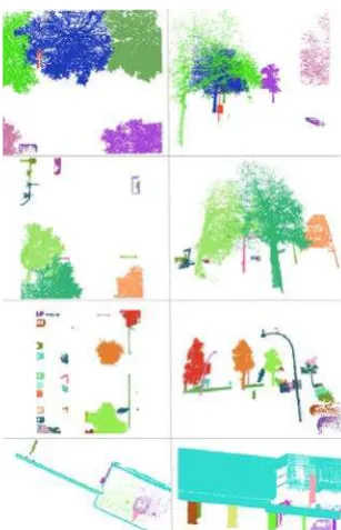
A test data set is manually created from the segmented dataset, to check the quality of the correlation measures for object detection and classification. The complete strip of 800 meter was labelled on 13 (sub) classes, and contains a total of 337 segments, see figure 8.
Figure 8 Test labels of 337 segments of 13 (sub) classes of a 800 m MLS dataset.
To test the ability to find all instances of a certain object, we have created sample components per class and analysed the correlation between these samples and all other components. For four classes the results are shown and discussed: lamp posts, traffic lights, cars and trees. Ideally, there is a threshold that separates all instances in a certain class from all the other objects. In practice, there may be false positives (incorrectly classified as being part of the class) or false negatives (objects from that a class are not detected as such). For all four detection results, a threshold is set. Components that are just below the threshold are also visualized to give an idea on which components are just not similar enough to be classified as such.
5.2.1 Lamp post detection
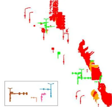
We identified four different types of lamp posts, so for each type one sample was selected an given the label of lamp posts (in grey inset in figure 9). For the lamp post samples, figure 9 shows all components that have a correlation higher than 0.8 with one of the lamp post samples. Red components are in the range of 0.8-0.85, and orange components are in between 0.85-The International Archives of the Photogrammetry, Remote Sensing and Spatial Information Sciences, Volume XL-3, 2014
0.9. All lamp posts in the test data are detected if the threshold is set at 0.8; however, eight other components are incorrectly recognized as lamp posts. At a correlation threshold of 0.9 only lamp posts are detected, however four are missed due to the tight threshold. It can be concluded that for lamp post there is no ideal threshold with this approach that detects all instances without having other classes included. A practical solution is to use a loose threshold, e.g. 0.8, and let the operator remove the false positives. In table 1, accuracy results are shown for the object detection of lamp posts, traffic signs, cars and trees.
Figure 9 Correlation results on four lamp post samples (inset). Components are coloured by correlation: >0.9 (green), >0.85 (orange) and <0.85 (red). Components with correlation lower
than 0.8 are not shown.
5.2.2 Traffic light detection
The traffic lights in our dataset consist of a combination of pole like objects, lamp posts and traffic signs. Still the correlation with other traffic lights is over 0.95 when the sample has the crossbar approximately at the same height. When using 4 sample components, only 2 test components were left, and two traffic signs are incorrectly detected as traffic light (figure 10).
Figure 10 Correlation results on traffic light samples (inset). Components are coloured by correlation: >0.95 (green), >0.9 (orange) and <0.9 (red). Components with correlation lower
than 0.85 are not shown.
5.2.3 Car detection
For cars, we selected four samples, of which two were moving and two were static. Figure 11 shows the result of the car detection based on the 4 car samples. With an acceptance threshold on the correlation of 0.9 six car components out of 134 were not detected as such: two insets are to show the reasons of these false negatives. The orange component has a correlation between 0.85-0.9. The dimensions of the component differ too much from the samples to be detected as car. The same holds for the van in the red lower inset. A solution for the user is to include this segment in the samples, with the risk of having including other segments that show similarities with this van. The 22 false positives mainly come from bicycles, fences and bushes. One of the samples actually is a component of half a car; many of the parked cars in our dataset are at the border of being cropped, leaving many components covering half of the car. This shows the flexibility of the user assisted approach, as all half-car components are now correctly classified as car.
Figure 11 Correlation results on car samples (inset). Components are coloured by correlation: >0.9 (green), >0.85 (orange) and <0.85 (red). Components with correlation lower
than 0.8 are not shown.
5.2.4 Tree detection
The variety of tree shapes is higher compared to the different shapes of road furniture and cars (figure 12).
Figure 12 Correlation results on tree samples (inset). Components are coloured by correlation:>0.8 (green), >0.75 (orange) and <0.75 (red). Components with correlation lower
than 0.7 are not shown.
For tree detection we used a lower acceptance threshold of 0.8 on the feature vector correlation. Another option would be to include more than 4 sample components. Still, with 4 samples 41 of 42 remaining trees are detected, together with 10 false positives. The only tree component that our algorithm missed is shown in the red inset. It is obvious that the component consist of multiple objects, including a fence and at least one tree. The ten false positives can be found in traffic lights and building facades.
An overview on the accuracy results of the detection of the four given classes are shown in table 1.
Class of sample
# sample
# test segmen ts
TP FN FP Correl
ation thresh old Lamp
post 4 22 18 4 0 0.9
Lamp
post 4 22 22 0 8 0.8
Traffic
light 4 2 2 0 2 0.95
Car 4 130 124 6 22 0.9
Tree 4 42 41 1 10 0.8
Table 1 Accuracy results for detecting objects using 4 samples per class.
Our interpretation of the results is that when looking at the false positives of all detection results, it should be relatively easy to automatically remove these from the results. One way could be based on the ICP algorithm, that checks on point based approach how similar two components are, or incorporate other feature attributes to rule out possibilities. Secondly, our method is not an automatic approach. This leaves it questionable what the accuracy measures mean. After all, if the operator selects a few samples more, the accuracy results will improve. So, it is not our aim to get a fantastic classification result, but to show that the method is generic enough to adapt to the local situation, and to the demands of the user.
5.3 Results of ICP algorithm for similar objects
Optional, an ICP algorithm can be performed to check whether sample and component are indeed corresponding to similar objects. At this moment, the results of the ICP algorithm are not integrated in the decision whether an object is detected or not; however, it can be shown to the user. In future work, a reliable measure based on the ICP results are used to detect attachments to certain objects, such as traffic signs to lamp posts as in figure 13.
Figure 13 Two components on lamp posts overlaid using relative coordinates (left) and after ICP algorithm (right).
5.4 Classification by fast selection of samples
The samples selected in the classification step are selected rather randomly; not all classes from the test data set are represented in the sample dataset, only the major classes. For example, pedestrians, roofs, flag poles and small traffic signs are not included. This directly increases the number of classification errors a little. The classification results are given in figures 14 and 15, and table 2. From table 2 we can conclude that mainly small segments are incorrectly classified, as 33% of the segments are incorrect, although they only represent 10% of the points.
Figure 14 Test dataset shown in 5 parts of about 150 m each. Points coloured by classification label (left), and whether that
agrees with the test label (green) or not (red) on the left.
Figure 15 Street view from part of the classified data (top) and corresponding correctness (bottom).
Correctness on TP FN % error
Segments 225 112 33.2
Points 1989k 238k 10.7
Table 2 Correctness on test dataset segmentwise and pointwise calculations.
The segmentation step including ground removal, point attributes calculations and connected component algorithm takes about 1 hour for this 20 Million point dataset. Although performances can be improved, normally a segmentation will be performed only once per dataset. Overnight, a 100 Million point dataset can be segmented. The processing time of the detection and classification stage are linear with the number of (points within) sample components. For the object detection using 4 samples on 337 components, the algorithm takes about 2-3 minutes. The classification using 22 samples takes about 10 minutes on a standard 2 GHz computer running under Windows.
6. OUTLOOK
In this paper it was shown that for a good object detection, a good segmentation is needed when following this approach. In order to further improve the segmentation, we get close to the point that we need to further integrate knowledge on the objects in the scene. Following this reasoning, an iterative approach between segmentation and classification sounds logical in improving both the segmentation and the classification. In future work our focus is on reducing the segmentation errors by using different point attributes and information of a pre-classification step. This can be in the form of removing all components that have a clear match with a sample component. The remaining components can be further analysed by subdividing them using the additional attributes in a mean-shift segmentation, or in case of over-segmentation try to group several components following the soup-of-segments approach of Malisiewicz and Efros (2007).
Calculation of the correlation is a standard way to calculate similarities. In case of noisy data, and objects attached to other objects, it is worth to analyse which parts of the vector contain the best information. In the future, a bag-of-words approach will be applied to be able to weight the attributes in the feature vector (Toldo et al, 2009). The weighting depends again on the class of the component.
The methodology is explained using a relatively small MLS dataset. When above mentioned further research possibilities have been explored, it is our goal to test the algorithm on bench mark datasets to analyse and compare our method with other approaches.
7. CONCLUSIONS
The main contribution of this paper is the use of point feature attributes to better segment MLS data into components that have a one-to-one relationship with objects.
The iterative growing algorithm presented in this paper showed that it is possible to distinguish individual trees even when their branches are connecting. There, the knowledge on how the density varies from bottom to top was successfully combined with how the segments should grow. The point feature on linearity was shown to be useful when separating objects which are connected by wires. When using an MMS that contains two scanners that capture the scene with a small time delay, the possibility arises to detect moving objects in the scene. This is done by using the attribute features on the local density of points, specially the number of points from the other sensor. The option to detect these dynamic objects helps to better interpret the point cloud, for example by deleting all moving objects if they are not of interest for a particular application. Although the segmentation is not free of errors, the similarity measures based on the height histograms and bounding box
properties proved to be sufficient to detect objects and to classify the MLS data. The approach to give some freedom to the user selecting components of interest and find similar ones, has the potential to be applied in many practical applications. For registration for example, the approach can be used in the task to find exactly the same objects.
REFERENCES
Beger, R., Gedrange, C., Hecht, R., Neubert, M., 2011. Data fusion of extremely high resolution aerial imagery and LiDAR data for automated railroad centre line reconstruction. ISPRS Journal of Photogrammetry and Remote Sensing, 66(6), S40-S51.
Brenner, C., 2009. Extraction of Features from Mobile Laser Scanning Data for Future Driver Assistance Systems Advances in GIScience. In M. Sester, L. Bernard & V. Paelke (Eds.), (pp. 25-42): Springer Berlin Heidelberg.
Bremer, M., Wichmann, V., and Rutzinger, M., 2013. Eigenvalue and graph-based object extraction from mobile laser scanning point clouds. In: ISPRS Ann. Photogramm. Remote Sens. Spatial Inf. Sci., II-5/W2, pp 55-60.
Kemboi, B., 2014. Knowledge based detection of road furniture objects in mobile laser scanner (MLS) data. MSc thesis, University of Twente Faculty of Geo-Information and Earth Observation (ITC).
Lai, K., and Fox, D., 2010. Object Recognition in 3D Point Clouds Using Web Data and Domain Adaptation. International Journal of Robotics Research 29(8), 1019-1037.
Malisiewicz, T., and Efros, A., 2007. Improving Spatial Support for Objects via Multiple Segmentations, BMCV 2007.
Oude Elberink, S., Khoshelham, K., Arastounia, M. and Diaz Benito, D., 2013. Rail Track Detection and Modelling in Mobile Laser Scanner Data. In: ISPRS Ann. Photogramm. Remote Sens. Spatial Inf. Sci., II-5/W2, pp 223-228.
Pu, S., Rutzinger, M., Vosselman, G., and Oude Elberink, S., 2011. Recognizing Basic Structures from Mobile Laser Scanning Data for Road Inventory Studies. ISPRS Journal of Photogrammetry and Remote Sensing, 66(6), S28-S39.
Toldo, R., Castellani, U. and Fusiello, A., 2009. A bag of words approach for 3d object categorization. In: MIRAGE’09. Velizhev, A., Shapovalov, R. and Schindler, K., 2012. Implicit shape models for object detection in 3D point clouds. In: ISPRS Ann. Photogramm. Remote Sens. Spatial Inf. Sci., I-3, pp 179-184.
Vosselman, G., 2013. Point cloud segmentation for urban scene classification. In: International Archives of the Photogrammetry, Remote Sensing and Spatial Information Sciences, Volume XL-7/W2, pp 257-262.