Klasifikasi. Data Mining

(1)

Klasifikasi

(2)

Klasifikasi

1 Decision Tree Induction 2 Bayesian Classification 3 Neural Network

4 Model Evaluation and Selection

(3)

(4)

1. Siapkan

data training

2. Pilih

atribut sebagai akar

3. Buat

cabang untuk tiap-tiap nilai

4. Ulangi proses

untuk setiap cabang sampai

semua kasus pada cabang memiliki kelas yg

sama

Tahapan Algoritma Decision Tree



   n i pi pi S Entropy 1 2 log * ) ( ) ( * | | | | ) ( ) , ( 1 i n i i S Entropy S S S Entropy A S Gain



  

(5)

(6)

• Untuk memilih atribut akar, didasarkan pada nilai Gain

tertinggi dari atribut-atribut yang ada. Untuk mendapatkan nilai Gain, harus ditentukan terlebih dahulu nilai Entropy • Rumus Entropy:

• S = Himpunan Kasus • n = Jumlah Partisi S

• pi = Proporsi dari Si terhadap S

• Rumus Gain:

• S = Himpunan Kasus • A = Atribut

• n = Jumlah Partisi Atribut A

• | Si | = Jumlah Kasus pada partisi ke-i

2. Pilih atribut sebagai akar



   n i pi pi S Entropy 1 2 log * ) ( ) ( * | | | | ) ( ) , ( 1 i n i i S Entropy S S S Entropy A S Gain



  

(7)

(8)

• Entropy Total

• Entropy (Outlook)

• Entropy (Temperature)

• Entropy (Humidity) • Entropy (Windy)

(9)

Penghitungan Entropy Akar

NODE ATRIBUT JML KASUS

(S) YA (Si)

TIDAK

(Si) ENTROPY GAIN

1 TOTAL 14 10 4 0,86312 OUTLOOK CLOUDY 4 4 0 0 RAINY 5 4 1 0,72193 SUNNY 5 2 3 0,97095 TEMPERATURE COOL 4 0 4 0 HOT 4 2 2 1 MILD 6 2 4 0,91830 HUMADITY HIGH 7 4 3 0,98523 NORMAL 7 7 0 0 WINDY FALSE 8 2 6 0,81128

(10)

(11)

Penghitungan Gain Akar

(S) YA (Si)

TIDAK

1 TOTAL 14 10 4 0,86312 OUTLOOK 0,25852 CLOUDY 4 4 0 0 RAINY 5 4 1 0,72193 SUNNY 5 2 3 0,97095 TEMPERATURE 0,18385 COOL 4 0 4 0 HOT 4 2 2 1 MILD 6 2 4 0,91830 HUMIDITY 0,37051 HIGH 7 4 3 0,98523 NORMAL 7 7 0 0 WINDY 0,00598 FALSE 8 2 6 0,81128 TRUE 6 4 2 0,91830

(12)

• Dari hasil pada Node 1, dapat diketahui bahwa atribut dengan Gain tertinggi adalah HUMIDITY yaitu sebesar 0.37051

• Dengan demikian HUMIDITY dapat menjadi node akar

• Ada 2 nilai atribut dari HUMIDITY yaitu HIGH dan NORMAL. Dari kedua nilai atribut tersebut, nilai atribut NORMAL sudah mengklasifikasikan kasus menjadi 1 yaitu keputusan-nya Yes, sehingga tidak perlu dilakukan perhitungan lebih lanjut

• Tetapi untuk nilai atribut HIGH masih perlu dilakukan perhitungan lagi

Gain Tertinggi Sebagai Akar

1. HUMIDITY

1.1

Yes

(13)

• Untuk memudahkan, dataset di-filter dengan

mengambil data yang memiliki kelembaban

HUMIDITY=HIGH untuk membuat Tabel Node 1.1

2. Buat cabang untuk tiap-tiap nilai

OUTLOOK TEMPERATURE HUMIDITY WINDY PLAY

Sunny Hot High FALSE No

Sunny Hot High TRUE No

Cloudy Hot High FALSE Yes

Rainy Mild High FALSE Yes

Sunny Mild High FALSE No

Cloudy Mild High TRUE Yes

(14)

Perhitungan Entropi Dan Gain Cabang

(S) YA (Si)

TIDAK

1.1 HUMIDITY 7 3 4 0,98523 OUTLOOK 0,69951 CLOUDY 2 2 0 0 RAINY 2 1 1 1 SUNNY 3 0 3 0 TEMPERATURE 0,02024 COOL 0 0 0 0 HOT 3 1 2 0,91830 MILD 4 2 2 1 WINDY 0,02024 FALSE 4 2 2 1 TRUE 3 1 2 0,91830

(15)

• Dari hasil pada Tabel Node 1.1, dapat diketahui bahwa atribut dengan Gain tertinggi adalah OUTLOOK yaitu

sebesar 0.69951

• Dengan demikian OUTLOOK dapat menjadi node kedua

• Artibut CLOUDY = YES dan SUNNY= NO sudah mengklasifikasikan kasus

menjadi 1 keputusan, sehingga tidak perlu dilakukan perhitungan lebih lanjut

• Tetapi untuk nilai atribut RAINY masih perlu dilakukan perhitungan lagi

Gain Tertinggi Sebagai Node 1.1

1. HUMIDITY 1.1 OUTLOOK Yes High _Normal Yes ????? 1.1.2 No Cloudy Rainy Sunny

(16)

3. Ulangi proses untuk setiap cabang sampai

semua kasus pada cabang memiliki kelas yg sama

OUTLOOK TEMPERATURE HUMIDITY WINDY PLAY

Rainy Mild High FALSE Yes

Rainy Mild High TRUE No

(S) YA (Si) TIDAK (Si) ENTROPY GAIN

1.1.2 HUMADITY HIGH &

OUTLOOK RAINY 2 1 1 1 TEMPERATURE 0 COOL 0 0 0 0 HOT 0 0 0 0 MILD 2 1 1 1 WINDY 1 FALSE 1 1 0 0 TRUE 1 0 1 0

(17)

• Dari tabel, Gain Tertinggi adalah WINDY dan

menjadi node cabang dari atribut RAINY

• Karena semua kasus

sudah masuk dalam kelas

• Jadi, pohon keputusan pada Gambar merupakan pohon keputusan terakhir yang terbentuk

Gain Tertinggi Sebagai Node 1.1.2

1. HUMIDIT Y 1.1 OUTLOOK Yes High _Normal Yes WINDY 1.1.2 No Cloudy Rainy Sunny Yes No False True

(18)

• Training data set:

Buys_computer

Decision Tree Induction: An Example

age income student credit_rating buys_computer

<=30 high no fair no <=30 high no excellent no 31…40 high no fair yes >40 medium no fair yes >40 low yes fair yes >40 low yes excellent no 31…40 low yes excellent yes <=30 medium no fair no <=30 low yes fair yes >40 medium yes fair yes <=30 medium yes excellent yes 31…40 medium no excellent yes 31…40 high yes fair yes >40 medium no excellent no

(19)

• Overfitting: An induced tree may overfit the training data

• Too many branches, some may reflect anomalies due to noise or outliers

• Poor accuracy for unseen samples

• Two approaches to avoid overfitting

1. Prepruning: Halt tree construction early ̵ do not split a node if this would result in the goodness measure falling below a threshold

• Difficult to choose an appropriate threshold

2. Postpruning: Remove branches from a “fully grown” tree

-get a sequence of progressively pruned trees

• Use a set of data different from the training data to decide which is the “best pruned tree”

(20)

(21)

• Relatively

faster learning speed

(than other

classification methods)

• Convertible to

simple and easy to understand

classification rules

• Can use

SQL queries for accessing databases

• Comparable classification accuracy

with

other methods

(22)

• Lakukan eksperimen untuk mengumpulkan

dataset yang memiliki 4-5 atribut dan analisis

dengan

decision tree

pada dataset tersebut.

(23)

(24)

• A

statistical classifier

: performs probabilistic prediction,

i.e., predicts class membership probabilities

• Foundation

: Based on Bayes’ Theorem.

• Performance

: A simple Bayesian classifier, naïve

Bayesian classifier, has comparable performance with

decision tree and selected neural network classifiers

• Incremental

: Each training example can incrementally

increase/decrease the probability that a hypothesis is

correct — prior knowledge can be combined with

observed data

• Standard

: Even when Bayesian methods are

computationally intractable, they can provide a

standard of optimal decision making against which

other methods can be measured

(25)

1. Baca Data Training

2. Hitung jumlah class

3. Hitung jumlah kasus yang sama dengan class

yang sama

4. Kalikan semua nilai hasil sesuai dengan data X

yang dicari class-nya

(26)

(27)

• X  Data dengan class yang belum diketahui

• H  Hipotesis data X yang merupakan suatu class yang lebih spesifik

• P (H|X)  Probabilitas hipotesis H berdasarkan kondisi X (posteriori probability)

• P (H)  Probabilitas hipotesis H (prior probability)

• P (X|H)  Probabilitas X berdasarkan kondisi pada hipotesis H • P (X)  Probabilitas X

Teorema Bayes

)

(

/

)

(

)

|

(

)

(

)

(

)

|

(

)

|

(

X

P

H

P

H

P

H

P

H

P

H

P





(28)

• Terdapat 2 class dari data training tersebut, yaitu:

• C1 (Class 1) Play = yes  9 record • C2 (Class 2) Play = no  5 record • Total = 14 record

• Maka:

• P (C1) = 9/14 = 0.642857143 • P (C2) = 5/14 = 0.357142857

• Pertanyaan:

• Data X = (outlook=rainy, temperature=cool, humidity=high, windy=true) • Naik gunung atau tidak?

(29)

• Untuk P(Ci) yaitu P(C1) dan P(C2) sudah diketahui

hasilnya di langkah sebelumnya.

• Selanjutnya Hitung P(X|Ci) untuk i = 1 dan 2

3. Hitung jumlah kasus yang sama dengan

class yang sama

(30)

• Jika semua atribut dihitung, maka didapat hasil

akhirnya seperti berikut ini:

3. Hitung jumlah kasus yang sama dengan

class yang sama

Atribute Parameter No Yes

Outlook value=sunny 0.6 0.2222222222222222 Outlook value=overcast 0.0 0.4444444444444444 Outlook value=rainy 0.4 0.3333333333333333 Temperature value=hot 0.4 0.2222222222222222 Temperature value=mild 0.4 0.4444444444444444 Temperature value=cool 0.2 0.3333333333333333 Humidity value=high 0.8 0.3333333333333333 Humidity value=normal 0.2 0.6666666666666666 Windy value=false 0.4 0.6666666666666666 Windy value=true 0.6 0.3333333333333333

(31)

• Pertanyaan:

• Data X = (outlook=rainy, temperature=cool, humidity=high, windy=true)

• Naik gunung atau tidak?

• Kalikan semua nilai hasil dari data X

• P(X|play=“yes”) = 0.333333333* 0.333333333* 0.333333333*0.333333333 = 0.012345679 • P(X|play=“no”) = 0.4*0.2*0.8*0.6=0.0384 • P(X|play=“yes”)*P(C1) = 0.012345679*0.642857143 = 0.007936508 • P(X|play=“no”)*P(C2) = 0.0384*0.357142857 = 0.013714286

• Nilai “no” lebih besar dari nilai “yes” maka class dari

4. Kalikan semua nilai hasil sesuai dengan

data X yang dicari class-nya

(32)

• Naïve Bayesian prediction requires each conditional prob. be non-zero. Otherwise, the predicted prob. will be zero

• Ex. Suppose a dataset with 1000 tuples, income=low (0), income= medium (990), and income = high (10)

• Use Laplacian correction (or Laplacian estimator) • Adding 1 to each case

Prob(income = low) = 1/1003

Prob(income = medium) = 991/1003 Prob(income = high) = 11/1003

• The “corrected” prob. estimates are close to their “uncorrected” counterparts

Avoiding the Zero-Probability Problem

   n k xk Ci P Ci X P 1 ) | ( ) | (

(33)

• Advantages

• Easy to implement

• Good results obtained in most of the cases

• Disadvantages

• Assumption: class conditional independence, therefore loss of accuracy

• Practically, dependencies exist among variables, e.g.:

• Hospitals Patients Profile: age, family history, etc.

• Symptoms: fever, cough etc.,

• Disease: lung cancer, diabetes, etc.

• Dependencies among these cannot be modeled by Naïve Bayes Classifier

• How to deal with these dependencies? Bayesian Belief Networks

(34)

(35)

• Neural Network adalah suatu model yang dibuat

untuk

meniru fungsi belajar yang dimiliki otak

manusia

atau jaringan dari sekelompok unit pemroses

kecil yang dimodelkan berdasarkan jaringan saraf

manusia

(36)

• Model Perceptron adalah model jaringan yang

terdiri dari beberapa unit masukan (ditambah

dengan sebuah bias), dan memiliki sebuah unit

keluaran

• Fungsi aktivasi bukan hanya merupakan fungsi

biner (0,1) melainkan bipolar (1,0,-1)

• Untuk suatu harga threshold ѳ yang ditentukan:

1 Jika net > ѳ

F (net) = 0 Jika – ѳ ≤ net ≤ ѳ -1 Jika net < - ѳ

(37)

Macam fungsi aktivasi yang dipakai untuk

mengaktifkan net di berbagai jenis neural network:

1. Aktivasi linear, Rumus:

y = sign(v) = v

2. Aktivasi step, Rumus:

3. Aktivasi sigmoid biner, Rumus: 4. Aktivasi sigmoid bipolar, Rumus:

(38)

1. Inisialisasi semua bobot dan bias (umumnya wi = b = 0)

2. Selama ada elemen vektor masukan yang respon unit keluarannya tidak sama dengan target, lakukan:

2.1 Set aktivasi unit masukan xi = Si (i = 1,...,n) 2.2 Hitung respon unit keluaran: net = + b

1 Jika net > ѳ

F (net) = 0 Jika – ѳ ≤ net ≤ ѳ

-1 Jika net < - ѳ

2.3 Perbaiki bobot pola yang mengadung kesalahan menurut persamaan: wi (baru) = wi (lama) + ∆w (i = 1,...,n) dengan ∆w = α t xi

b (baru) = b(lama) + ∆ b dengan ∆b = α t

Dimana: α = Laju pembelajaran (Learning rate) yang ditentukan ѳ = Threshold yang ditentukan

t = Target

2.4 Ulangi iterasi sampai perubahan bobot (∆wn = 0) tidak ada

Semakin besar α, semakin sedikit iterasi. Namun, α terlalu besar akan

Tahapan Algoritma Perceptron

(39)

• Diketahui sebuah dataset kelulusan berdasarkan

IPK untuk program S1:

• Jika ada mahasiswa

IPK 2.85 dan masih semester 1

,

maka masuk ke dalam manakah status tersebut ?

Studi Kasus

Status IPK Semester

Lulus 2.9 1 Tidak Lulus 2.8 3 Tidak Lulus 2.3 5 Tidak lulus 2.7 6

(40)

• Inisialisasi Bobot dan bias awal:

b = 0

dan

bias = 1

1: Inisialisasi Bobot

t X1 X2 1 2,9 1 -1 2.8 3 -1 2.3 5 -1 2,7 6

(41)

• Treshold (batasan), θ = 0 , yang artinya :

1 Jika net > 0

F (net) =

0 Jika net = 0

-1

Jika net < 0

(42)

• Hitung Response Keluaran iterasi 1

• Perbaiki bobot pola yang mengandung kesalahan

2.2 - 2.3 Hitung Respon dan Perbaiki

Bobot

MASUKAN TARGET y= PERUBAHAN BOBOT BOBOT BARU

X1 X2 1 t NET f(NET) ∆W1 ∆W2 ∆b W1 W2 b INISIALISASI 0 0 0 2,9 1 1 1 0 0 2.9 1 1 2.9 1 1 2,8 3 1 -1 12.12 1 -2.8 -3 -1 0.1 -2 0 2,3 5 1 -1 -9.77 -1 0 0 0 0.1 -2 0 2,7 6 1 -1 -11.7 -1 0 0 0 0.1 -2 0

(43)

• Hitung Response Keluaran iterasi 2

• Perbaiki bobot pola yang mengandung kesalahan

2.4 Ulangi iterasi sampai perubahan bobot

(∆wn = 0) tidak ada (Iterasi 2)

X1 X2 1 t NET f(NET) ∆W1 ∆W2 ∆b W1 W2 b INISIALISASI 0.1 -2 0 2,9 1 1 1 -1.71 -1 2.9 1 1 3 -1 1 2,8 3 1 -1 6.4 1 -2.8 -3 -1 0.2 -4 0 2,3 5 1 -1 -19.5 -1 0 0 0 0.2 -4 0 2,7 6 1 -1 -23.5 -1 0 0 0 0.2 -4 0

(44)

• Hitung Response Keluaran iterasi 3

• Perbaiki bobot pola yang mengandung kesalahan

• Semua pola f(net) = target, maka jaringan sudah mengenal semua pola dan iterasi dihentikan.

• Untuk data IPK memiliki pola 3.2 x - 5 y + 1 = 0 dapat dihitung prediksinya menggunakan bobot yang terakhir didapat:

2.4 Ulangi iterasi sampai perubahan bobot

(∆wn = 0) tidak ada .... (Iterasi 5)

X1 X2 1 t NET f(NET) ∆W1 ∆W2 ∆b W1 W2 b INISIALISASI 3.2 -5 1 2,9 1 1 1 5.28 1 0 0 0 3.2 -5 1 2,8 3 1 -1 -5.04 -1 0 0 0 3.2 -5 1 2,3 5 1 -1 -16.6 -1 0 0 0 3.2 -5 1 2,7 6 1 -1 -20.4 -1 0 0 0 3.2 -5 1

(45)

• Lakukan eksperimen untuk mengumpulkan

dataset yang memiliki 4-5 atribut dan analisis

dengan

Naïve Bayes

dan neural network

pada dataset tersebut

(46)

(47)

• Evaluation metrics

: How can we measure accuracy?

Other metrics to consider?

• Use validation test set of class-labeled tuples

instead of training set when assessing accuracy

• Methods for estimating a

classifier’s accuracy

:

• Holdout method, random subsampling

• Cross-validation • Bootstrap

• Comparing

classifiers:

• Confidence intervals

• Cost-benefit analysis and ROC Curves

(48)

• Holdout method

• Given data is randomly partitioned into two independent sets

• Training set (e.g., 2/3) for model construction

• Test set (e.g., 1/3) for accuracy estimation • Random sampling: a variation of holdout

• Repeat holdout k times, accuracy = avg. of the accuracies obtained

• Cross-validation (k-fold, where k = 10 is most popular) • Randomly partition the data into k mutually exclusive

subsets, each approximately equal size

• At i-th iteration, use D_ias test set and others as training set • Leave-one-out: k folds where k = # of tuples, for small sized

data

• *Stratified cross-validation*: folds are stratified so that class dist. in each fold is approx. the same as that in the initial

Evaluating Classifier Accuracy:

(49)

• Bootstrap

• Works well with small data sets

• Samples the given training tuples uniformly with replacement, i.e., each time a tuple is selected, it is equally likely to be selected again and re-added to the training set

• Several bootstrap methods, and a common one is .632 boostrap

1. A data set with d tuples is sampled d times, with replacement, resulting in a training set of d samples

2. The data tuples that did not make it into the training set end up forming the test set. About 63.2% of the original data end up in the bootstrap, and the remaining 36.8% form the test set (since (1 – 1/d)d

≈ e-1_{= 0.368)}

3. Repeat the sampling procedure k times, overall accuracy of the model:

(50)

• Suppose we have two classifiers,

M

₁

and M

₂

,

which one is better

?

• Use 10-fold cross-validation to obtain and

• These mean error rates are just estimates of error on the true

population of future data cases

• What if the difference between the two error rates is just attributed to chance?

• Use a test of statistical significance

• Obtain confidence limits for our error estimates

Estimating Confidence Intervals:

(51)

1. Perform 10-fold cross-validation

2. Assume samples follow a

t distribution

with k–1

degrees of freedom

(here, k=10)

3. Use

t-test

(or

Student’s t-test

)

4. Null Hypothesis

: M

₁

& M

₂

are the same

5. If we can

reject

null hypothesis, then

1. we conclude that the difference between M₁ & M₂ is

statistically significant

2. Chose model with lower error rate

Estimating Confidence Intervals:

Null Hypothesis

(52)

• If only 1 test set available:

pairwise comparison

• For ith_{round of 10-fold cross-validation, the same cross} partitioning is used to obtain err(M₁)_i and err(M₂)_i

• Average over 10 rounds to get

• t-test computes t-statistic with k-1 degrees of freedom:

• If two test sets available: use

non-paired t-test

Estimating Confidence Intervals: t-test

where

(53)

Estimating Confidence Intervals:

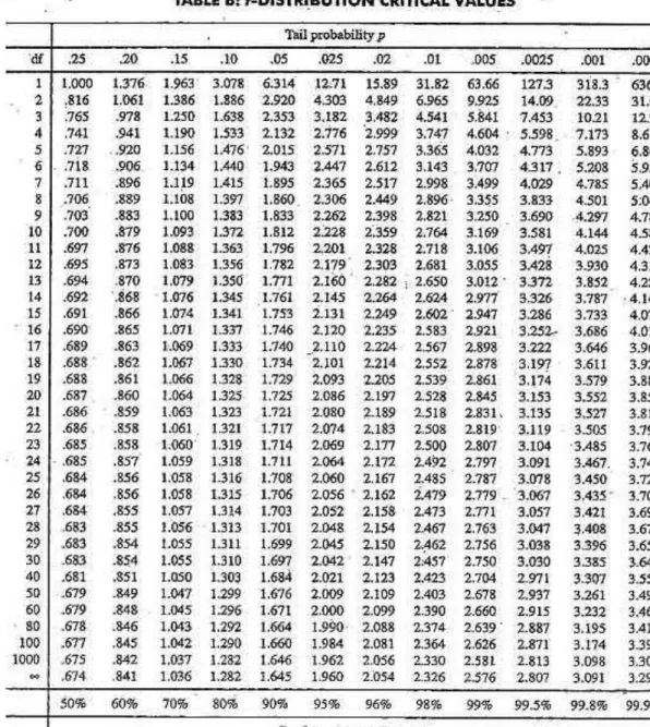
Table for t-distribution

• Symmetric

• Significance level, e.g., sig

= 0.05 or 5% means M₁ & M₂ are significantly

different for 95% of

population

(54)

Are M₁ & M₂ significantly different?

1. Compute t. Select significance level (e.g. sig = 5%) 2. Consult table for t-distribution: Find t value

corresponding to k-1 degrees of freedom (here, 9)

3. t-distribution is symmetric: typically upper % points of distribution shown → look up value for confidence limit z=sig/2 (here, 0.025)

4. If t > z or t < -z, then t value lies in rejection region:

1. Reject null hypothesis that mean error rates of M₁ & M₂ are same

2. Conclude: statistically significant difference between M₁ & M₂

5. Otherwise, conclude that any difference is chance

Estimating Confidence Intervals:

(55)

• ROC (Receiver Operating

Characteristics) curves: for visual comparison of classification models

• Originated from signal detection theory

• Shows the trade-off between the true positive rate and the false positive rate • The area under the ROC curve is a

measure of the accuracy of the model

• Rank the test tuples in decreasing order: the one that is most likely to belong to the positive class appears at the top of the list

• The closer to the diagonal line (i.e., the closer the area is to 0.5), the less

accurate is the model

• Vertical axis represents the true positive rate

• Horizontal axis rep. the false positive rate

• The plot also shows a diagonal line

(56)

• Accuracy

• classifier accuracy: predicting class label

• Speed

• time to construct the model (training time)

• time to use the model (classification/prediction time)

• Robustness: handling noise and missing values

• Scalability: efficiency in disk-resident databases

• Interpretability

• understanding and insight provided by the model

• Other measures, e.g., goodness of rules, such as decision tree size or compactness of classification rules

(57)

5 Techniques to Improve

Classification Accuracy: Ensemble

Methods

(58)

• Ensemble methods

• Use a combination of models to increase accuracy

• Combine a series of k learned models, M1, M2, …, Mk, with the aim of creating an improved model M*

• Popular ensemble methods

• Bagging: averaging the prediction over a collection of classifiers

• Boosting: weighted vote with a collection of classifiers

• Ensemble: combining a set of heterogeneous classifiers

(59)

• Analogy: Diagnosis based on multiple doctors’ majority vote

• Training

• Given a set D of d tuples, at each iteration i, a training set D_i of d tuples is sampled with replacement from D (i.e., bootstrap)

• A classifier model M_i is learned for each training set D_i

• Classification: classify an unknown sample X • Each classifier M_i returns its class prediction

• The bagged classifier M* counts the votes and assigns the class with the most votes to X

• Prediction: can be applied to the prediction of continuous values by taking the average value of each prediction for a given test tuple

• Accuracy

• Often significantly better than a single classifier derived from D • For noise data: not considerably worse, more robust

(60)

• Analogy: Consult several doctors, based on a combination of

weighted diagnoses—weight assigned based on the previous

diagnosis accuracy • How boosting works?

1. Weights are assigned to each training tuple

2. A series of k classifiers is iteratively learned

3. After a classifier M_i is learned, the weights are updated to allow the subsequent classifier, M_i+1, to pay more attention

to the training tuples that were misclassified by M_i

4. The final M* combines the votes of each individual

classifier, where the weight of each classifier's vote is a function of its accuracy

• Boosting algorithm can be extended for numeric prediction

• Comparing with bagging: Boosting tends to have greater accuracy, but it also risks overfitting the model to misclassified data

(61)

1. Given a set of d class-labeled tuples, (X₁, y₁), …, (X_d, y_d) 2. Initially, all the weights of tuples are set the same (1/d) 3. Generate k classifiers in k rounds. At round i,

1. Tuples from D are sampled (with replacement) to form a training set D_i of the same size

2. Each tuple’s chance of being selected is based on its weight 3. A classification model M_i is derived from D_i

4. Its error rate is calculated using D_ias a test set

5. If a tuple is misclassified, its weight is increased, o.w. it is decreased

4. Error rate: err(X_j) is the misclassification error of tuple X_j. Classifier M_i error rate is the sum of the weights of the misclassified tuples:

Adaboost (Freund and Schapire, 1997)

) ( 1error M



  d j j i w err M error( ) (X_j)

(62)

• Random Forest:

• Each classifier in the ensemble is a decision tree classifier and is generated using a random selection of attributes at each node to determine the split

• During classification, each tree votes and the most popular class is returned

• Two Methods to construct Random Forest:

1. Forest-RI (random input selection): Randomly select, at each node, F attributes as candidates for the split at the node. The CART methodology is used to grow the trees to maximum size

2. Forest-RC (random linear combinations): Creates new attributes

(or features) that are a linear combination of the existing

attributes (reduces the correlation between individual classifiers)

• Comparable in accuracy to Adaboost, but more robust to errors and outliers

• Insensitive to the number of attributes selected for consideration at each split, and faster than bagging or

(63)

• Class-imbalance problem: Rare positive example but

numerous negative ones, e.g., medical diagnosis, fraud, oil-spill, fault, etc.

• Traditional methods assume a balanced distribution of classes and equal error costs: not suitable for

class-imbalanced data

• Typical methods for imbalance data in 2-class classification:

1. Oversampling: re-sampling of data from positive class

2. Under-sampling: randomly eliminate tuples from negative class

3. Threshold-moving: moves the decision threshold, t, so that the rare class tuples are easier to classify, and