Greening Geographical Load Balancing
Zhenhua Liu, Minghong Lin,
Adam Wierman, Steven H. Low
CMS, California Institute of Technology, Pasadena{zliu2,mhlin,adamw,slow}@caltech.edu
Lachlan L. H. Andrew
Faculty of ICTSwinburne University of Technology, Australia
[email protected]
ABSTRACT
Energy expenditure has become a significant fraction of data center operating costs. Recently, “geographical load balanc-ing” has been suggested to reduce energy cost by exploiting the electricity price differences across regions. However, this reduction of cost can paradoxically increase total energy use. This paper explores whether the geographical diversity of Internet-scale systems can additionally be used to provide environmental gains. Specifically, we explore whether geo-graphical load balancing can encourage use of “green” renew-able energy and reduce use of “brown” fossil fuel energy. We make two contributions. First, we derive two distributed al-gorithms for achieving optimal geographical load balancing. Second, we show that if electricity is dynamically priced in proportion to the instantaneous fraction of the total energy that is brown, then geographical load balancing provides sig-nificant reductions in brown energy use. However, the ben-efits depend strongly on the degree to which systems accept dynamic energy pricing and the form of pricing used.
Categories and Subject Descriptors
C.2.4 [Computer-Communication Networks]: Distributed Systems
General Terms
Algorithms, Performance
1.
INTRODUCTION
Increasingly, web services are provided by massive, geo-graphically diverse “Internet-scale”distributed systems, some having several data centers each with hundreds of thousands of servers. Such data centers require many megawatts of electricity and so companies like Google and Microsoft pay tens of millions of dollars annually for electricity [31].
The enormous, and growing energy demands of data cen-ters have motivated research both in academia and industry on reducing energy usage, for both economic and environ-mental reasons. Engineering advances in cooling, virtualiza-tion, multi-core servers, DC power, etc. have led to signifi-cant improvements in the Power Usage Effectiveness (PUE) of data centers; see [6, 37, 19, 21]. Such work focuses on re-ducing theenergy use of data centers and their components.
Permission to make digital or hard copies of all or part of this work for personal or classroom use is granted without fee provided that copies are not made or distributed for profit or commercial advantage and that copies bear this notice and the full citation on the first page. To copy otherwise, to republish, to post on servers or to redistribute to lists, requires prior specific permission and/or a fee.
SIGMETRICS’11, June 7–11, 2011, San Jose, California, USA.
Copyright 2011 ACM 978-1-4503-0262-3/11/06 ...$10.00.
A different stream of research has focused on exploiting the geographical diversity of Internet-scale systems to re-duce theenergy cost. Specifically, a system with clusters at tens or hundreds of locations around the world can dynam-ically route requests/jobs to clusters based on proximity to the user, load, and local electricity price. Thus, dynamic ge-ographical load balancing can balance the revenue lost due to increased delay against the electricity costs at each location. In recent years, many papers have illustrated the poten-tial of geographical load balancing to provide significant cost savings for data centers, e.g., [24, 28, 31, 32, 34, 39] and the references therein. The goal of the current paper is differ-ent. Our goal is to explore the social impact of geographical load balancing systems. In particular, geographical load bal-ancing aims to reduce energy costs, but this can come at the expense of increased total energy usage: by routing to a data center farther from the request source to use cheaper energy, the data center may need to complete the job faster, and so use more service capacity, and thus energy, than if the request was served closer to the source.
In contrast to this negative consequence, geographical load balancing also provides a huge opportunity for environmental benefit as the penetration of green, renewable energy sources increases. Specifically, an enormous challenge facing the elec-tric grid is that of incorporating intermittent, unpredictable renewable sources such as wind and solar. Because genera-tion supplied to the grid must be balanced by demand (i) in-stantaneously and (ii) locally (due to transmission losses), renewable sources pose a significant challenge. A key tech-nique for handling the unpredictability of renewable sources
isdemand-response, which entails the grid adjusting the
de-mand by changing the electricity price [2]. However, dede-mand response entails alocal customer curtailing use. In contrast, the demand of Internet-scale systems is flexible geographi-cally; thus traffic can be routed to different regions to “follow the renewables”, providing demand-response without service interruption. Since data centers represent a significant and growing fraction of total electricity consumption, and the IT infrastructure is already in place, geographical load balanc-ing has the potential to provide an extremely inexpensive approach for enabling large scale, global demand-response.
The key to realizing the environmental benefits above is for data centers to move from the fixed price contracts that are now typical toward some degree of dynamic pricing, with lower prices when green energy is available. The demand response markets currently in place provide a natural way for this transition to occur, and there is already evidence of some data centers participating in such markets [2].
Contribution (1): To derive distributed geographical load balancing algorithms we use a simple but general model, described in detail in Section 2. In it, each data center mini-mizes its cost, which is a linear combination of an energy cost and the lost revenue due to the delay of requests (which in-cludes both network propagation delay and load-dependent queueing delay within a data center). The geographical load balancing algorithm must then dynamically define both how requests should be routed to data centers and how to allo-cate capacity in each data center (i.e., how many servers are kept in active/energy-saving states).
In Section 3, we characterize the optimal geographical load balancing solutions and show that they have practically ap-pealing properties, such as sparse routing tables. Then, in Section 4, we use the previous characterization to give two distributed algorithms which provably compute the optimal routing and provisioning decisions, and which require differ-ent types of coordination of computation. Finally, we eval-uate the distributed algorithms in a trace-driven numeric simulation of a realistic, distributed, Internet-scale system (Section 5). The results show that a cost saving of over 40% during light-traffic periods is possible.
Contribution (2): In Section 6 we evaluate the feasibility and benefits of using geographical load balancing to facilitate the integration of renewable sources into the grid. We do this using a trace-driven numeric simulation of a realistic, distributed Internet-scale system in combination with models for the availability of wind and solar energy over time.
When the data center incentive is aligned with the social objective or reducing brown energy by dynamically pricing electricity proportionally to the fraction of the total energy coming from brown sources, we show that “follow the renew-ables” routing ensues (see Figure 5), causing significant social benefit. In contrast, we also determine the wasted brown en-ergy when prices are static, or are dynamic but do not align data center and social objectives.
2.
MODEL AND NOTATION
We now introduce the workload and data center models, followed by the geographical load balancing problem.
2.1
The workload model
We consider a discrete-time model whose timeslot matches the timescale at which routing decisions and capacity provi-sioning decisions can be updated. There is a (possibly long) interval of interestt∈ {1, . . . , T}. There are|J| geographi-cally concentrated sources of requests, i.e., “cities”, and the mean arrival rate from sourcejat timetisLj(t). Job
inter-arrival times are assumed to be much shorter than a timeslot, so that provisioning can be based on the average arrival rate during a slot. In practice, T could be a month and a slot length could be 1 hour. Our analytic results make no as-sumptions on Lj(t); however to provide realistic estimates
we use real-world traces to defineLj(t) in Sections 5 and 6.
2.2
The data center cost model
We model an Internet-scale system as a collection of |N|
geographically diverse data centers, where data center i is modeled as a collection of Mi homogeneous servers. The
model focuses on two key control decisions of geographical load balancing: (i) determiningλij(t), the amount of traffic
routed from sourcej to data center i; and (ii) determining
mi(t) ∈ {0, . . . , Mi}, the number of active servers at data
centeri. The system seeks to chooseλij(t) andmi(t) in order
to minimize cost during [1, T]. Depending on the system design these decisions may be centralized or decentralized. Algorithms for these decisions are the focus of Section 4.
Our model for data center costs focuses on the server costs of the data center.1 We model costs by combining theenergy cost and thedelay cost(in terms of lost revenue). Note that, to simplify the model, we do not include the switching costs associated with cycling servers in and out of power-saving modes; however the approach of [24] provides a natural way to incorporate such costs if desired.
Energy cost. To capture the geographic diversity and variation over time of energy costs, we let gi(t, mi, λi)
de-note the energy cost for data centeriduring timeslottgiven
miactive servers and arrival rateλi. For every fixedt, we
as-sume thatgi(t, mi, λi) is continuously differentiable in both
mi and λi, strictly increasing in mi, non-decreasing in λi,
and convex in mi. This formulation is quite general, and
captures, for example, the common charging plan of a fixed price per kWh plus an additional “demand charge” for the peak of the average power used over a sliding 15 minute win-dow [27]. Additionally, it can capture a wide range of models for server power consumption, e.g., energy costs as an affine function of the load, see [14], or as a polynomial function of the speed, see [40, 5].
Definingλi(t) =Pj∈Jλij(t), the total energy cost of data
centeriduring timeslott,Ei(t), is simply
Ei(t) =gi(t, mi(t), λi(t)). (1)
Delay cost. The delay cost captures the lost revenue incurred because of the delay experienced by the requests. To model this, we definer(d) as the lost revenue associated with a job experiencing delay d. We assume that r(d) is strictly increasing and convex ind.
To model the delay, we consider its two components: the network delay experienced while the request is outside of the data center and the queueing delay experienced while the request is at the data center.
To model thenetwork delay, we letdij(t) denote the
net-work delay experienced by a request from source jto data centeriduring timeslott. We make no requirements on the structure of thedij(t).
To model thequeueing delay, we letfi(mi, λi) denote the
queueing delay at data center igiven mi active servers and
an arrival rate ofλi. We assume thatfiis strictly decreasing
in mi, strictly increasing inλi, and strictly convex in both
miandλi. Further, for stability, we must have thatλi= 0 or
λi< miµi, whereµiis the service rate of a server at data
cen-teri. Thus, we definefi(mi, λi) =∞for λi ≥miµi.
Else-where, we assumefi is finite, continuous and differentiable.
Note that these assumptions are satisfied by most standard queueing formulae, e.g., the mean delay under M/GI/1 Pro-cessor Sharing (PS) queue and the 95th percentile of delay under the M/M/1. Further, the convexity offiinmimodels
the law of diminishing returns for parallelism.
Combining the above gives the following model for the total delay costDi(t) at data centeriduring timeslott:
Di(t) =
X
j∈Jλij(t)r(fi(mi(t), λi(t)) +dij(t)). (2)
2.3
The geographical load balancing problem
Given the cost models above, the goal of geographical load balancing is to choose the routing policyλij(t) and the
num-ber of active servers in each data center mi(t) at each time
tin order minimize the total cost during [1, T]. This is cap-tured by the following optimization problem:
min
m(t),λ(t)
XT
t=1 X
i∈N(Ei(t) +Di(t)) (3a)
s.t. X
i∈Nλij(t) =Lj(t), ∀j∈J (3b)
λij(t)≥0, ∀i∈N,∀j∈J (3c)
0≤mi(t)≤Mi, ∀i∈N (3d)
mi(t)∈N, ∀i∈N (3e)
To simplify (3), note that Internet data centers typically con-tain thousands of active servers. So, we can relax the integer constraint in (3) and round the resulting solution with min-imal increase in cost. Also, because this model neglects the cost of turning servers on or off, the optimization decouples into independent sub-problems for each timeslot t. For the analysiswe consider only a single interval and omit the
ex-plicit time dependence.2 Thus (3) becomes
min
m,λ
X
i∈N
gi(mi, λi) +
X
i∈N
X
j∈J
λijr(dij+fi(mi, λi)) (4a)
s.t. X
i∈Nλij=Lj, ∀j∈J (4b)
λij≥0, ∀i∈N,∀j∈J (4c)
0≤mi≤Mi, ∀i∈N, (4d)
We refer to this formulation as GLB. Note that GLB is jointly convex in λij and mi and can be efficiently solved
centrally. However, a distributed solution algorithm is usu-ally required, such as those derived in Section 4.
In contrast to prior work studying geographical load bal-ancing, it is important to observe that this paper is the first, to our knowledge, to incorporate jointly optimizing the total energy cost and the end-to-end user delay with consideration of both price diversity and network delay diversity.
GLB provides a general framework for studying geographi-cal load balancing. However, the model ignores many aspects of data center design, e.g., reliability and availability, which are central to data center service level agreements. Such is-sues are beyond the scope of this paper; however our designs merge nicely with proposals such as [36] for these goals.
The GLB model is too broad for some of our analytic re-sults and thus we often use two restricted versions.
Linear lost revenue. This model uses a lost revenue function r(d) = βd, for constant β. Though it is difficult to choose a “universal” form for the lost revenue associated with delay, there is evidence that it is linear within the range of interest for sites such as Google, Bing, and Shopzilla [13]. GLB then simplifies to
min
m,λ
X
i∈N
gi(mi, λi)+β
X
i∈N
λifi(mi, λi) +
X
i∈N
X
j∈J
dijλij
! (5)
subject to (4b)–(4d). We call this optimization GLB-LIN.
Queueing-based delay.We occasionally specify the form off andgusing queueing models. This provides increased intuition about the distributed algorithms presented.
If the workload is perfectly parallelizable, and arrivals are Poisson, then fi(mi, λi) is the average delay of mi
paral-lel queues, each with arrival rateλi/mi. Moreover, if each
queue is an M/GI/1 Processor Sharing (PS) queue, then
fi(mi, λi) = 1/(µi−λi/mi). We also assume gi(mi, λi) =
pimi, which implies that the increase in energy cost per
timeslot for being in an active state, rather than a low-power state, ismiregardless ofλi.
Under these restrictions, the GLB formulation becomes:
min
m,λ
X
i∈N
pimi+β
X
j∈J
X
i∈N
λij
1
µi−λi/mi +dij
(6a)
2Time-dependence ofL
jand prices is re-introduced for, and
central to, the numeric results in Sections 5 and 6.
subject to (4b)–(4d) and the additional constraint
λi≤miµi ∀i∈N. (6b)
We refer to this optimization as GLB-Q.
Additional Notation. Throughout the paper we use|S|
to denote the cardinality of a setS and bold symbols to de-note vectors or tuples. In particular,λj= (λij)i∈N denotes
the tuple ofλij from sourcej, andλ−j = (λik)i∈N,k∈J\{j}
denotes the tuples of the remainingλik, which forms a
ma-trix. Similarlym= (mi)i∈N andλ= (λij)i∈N,j∈J.
We also need the following in discussing the algorithms. Define Fi(mi, λi) = gi(mi, λi) +βλifi(mi, λi), and define
F(m,λ) =P
i∈NFi(mi, λi) + Σijλijdij. Further, let ˆmi(λi)
be the unconstrained optimalmiat data centerigiven fixed
λi, i.e., the unique solution to∂Fi(mi, λi)/∂mi= 0.
2.4
Practical considerations
Our model assumes there exist mechanisms for dynami-cally (i) provisioning capacity of data centers, and (ii) adapt-ing the routadapt-ing of requests from sources to data centers.
With respect to (i), many dynamic server provisioning techniques are being explored by both academics and indus-try, e.g., [4, 11, 16, 38]. With respect to (ii), there are also a variety of protocol-level mechanisms employed for data cen-ter selection today. They include, (a) dynamically generated DNS responses, (b) HTTP redirection, and (c) using per-sistent HTTP proxies to tunnel requests. Each of these has been evaluated thoroughly, e.g., [12, 25, 30], and though DNS has drawbacks it remains the preferred mechanism for many industry leaders such as Akamai, possibly due to the added latency due to HTTP redirection and tunneling [29]. Within the GLB model, we have implicitly assumed that there exists a proxy/DNS server co-located with each source.
Our model also assumes that the network delays,dij can
be estimated, which has been studied extensively, including work on reducing the overhead of such measurements, e.g., [35], and mapping and synthetic coordinate approaches, e.g., [22, 26]. We discuss the sensitivity of our algorithms to error in these estimates in Section 5.
3.
CHARACTERIZING THE OPTIMA
We now provide characterizations of the optimal solutions to GLB, which are important for proving convergence of the distributed algorithms of Section 4. They are also necessary because, a priori, one might worry that the optimal solu-tion requires a very complex routing structure, which would be impractical; or that the set of optimal solutions is very fragmented, which would slow convergence in practice. The results here show that such worries are unwarranted.
Uniqueness of optimal solution.
To begin, note that GLB has at least one optimal solu-tion. This can be seen by applying Weierstrass theorem [7], since the objective function is continuous and the feasible set is compact subset of Rn. Although the optimal solution is generally not unique, there are natural aggregate quantities unique over the set of optimal solutions, which is a convex set. These are the focus of this section.
A first result is that for the GLB-LIN formulation, under weak conditions on fi and gi, we have that λi is common
across all optimal solutions. Thus, the input to the data center provisioning optimization is unique.
Theorem 1. Consider the GLB-LIN formulation. Sup-pose that for alli,Fi(mi, λi) is jointly convex inλiandmi,
and continuously differentiable in λi. Further, suppose that
ˆ
mi(λi)is strictly convex. Then, for eachi,λiis common for
The proof is in the Appendix. Theorem 1 implies that the server arrival rates at each data center, i.e.,λi/mi, are
common among all optimal solutions.
Though the conditions on Fi and ˆmi are weak, they do
not hold for GLB-Q. In that case, ˆmi(λi) is linear, and thus
not strictly convex. Although theλiare not common across
all optimal solutions in this setting, the server arrival rates remain common across all optimal solutions.
Theorem 2. For each data center i, the server arrival
rates, λi/mi, are common across all optimal solutions to
GLB-Q.
Sparsity of routing.
It would be impractical if the optimal solutions to GLB required that traffic from each source was divided up among (nearly) all of the data centers. In general, eachλijcould be
non-zero, yielding|N| × |J| flows of traffic from sources to data centers, which would lead to significant scaling issues. Luckily, there is guaranteed to exist an optimal solution with extremely sparse routing. Specifically:
Theorem 3. There exists an optimal solution to GLB with at most(|N|+|J| −1)of theλij strictly positive.
Though Theorem 3 does not guarantee that every optimal solution is sparse, the proof is constructive. Thus, it pro-vides an approach which allows one to transform an optimal solution into a sparse optimal solution.
The following result further highlights the sparsity of the routing: any source will route to at most one data center that is not fully active, i.e., where there exists at least a server in power-saving mode.
Theorem 4. Consider GLB-Q where power costspi are
drawn from an arbitrary continuous distribution. If any source
j∈J has its traffic split between multiple data centersN′⊆
N in an optimal solution, then, with probability 1, at most
one data centeri∈N′ hasmi< Mi.
4.
ALGORITHMS
We now focus on GLB-Q and present two distributed al-gorithms that solve it, and prove their convergence.
Since GLB-Q is convex, it can be efficiently solved cen-trally if all necessary information can be collected at a single point, as may be possible if all the proxies and data cen-ters were owned by the same system. However there is a strong case for Internet-scale systems to outsource route se-lection [39]. To meet this need, the algorithms presented be-low are decentralized and albe-low each data center and proxy to optimize based on partial information.
These algorithms seek to fill a notable hole in the grow-ing literature on algorithms for geographical load balancgrow-ing. Specifically, they have provable optimality guarantees for a performance objective that includes both energy and delay, where route decisions are made using both energy price and network propagation delay information. The most closely related work [32] investigates the total electricity cost for data centers in a multi-electricity-market environment. It contains the queueing delay inside the data center (assumed to be an M/M/1 queue) but neglects the end-to-end user delay. Conversely, [39] uses a simple, efficient algorithm to coordinate the “replica-selection” decisions, but assumes the capacity at each data center is fixed. Other related works, e.g., [32, 34, 28], either do not provide provable guarantees or ignore diverse network delays and/or prices.
Algorithm 1: Gauss-Seidel iteration
Algorithm 1 is motivated by the observation that GLB-Q is separable in mi, and, less obviously, also separable in
λj := (λij, i∈N). This allows all data centers as a group
and each proxy jto iteratively solve for optimal mand λj
in a distributed manner, and communicate their intermedi-ate results to each other. Though distributed, Algorithm 1 requires each proxy to solve an optimization problem.
To highlight the separation between data centers and prox-ies, we reformulate GLB-Q as:
min
λj∈Λj
min
mi∈Mi
X
i∈N
pimi+ βλi
µi−λi/mi
+βX
i,j
λijdij (7)
Mi := [0, Mi] Λj := {λj|λj≥0,
X
i∈N
λij=Lj} (8)
Since the objective and constraintsMiand Λjare separable,
this can be solved separately by data centersiand proxiesj. The iterations of the algorithm are indexed byτ, and are assumed to be fast relative to the timeslotst. Each iteration
τ is divided into|J|+ 1 phases. In phase 0, all data centersi
concurrently calculatemi(τ+ 1) based on their own arrival
ratesλi(τ), by minimizing (7) over their own variablesmi:
min
mi∈Mi
pimi+ βλi(τ)
µi−λi(τ)/mi
(9)
In phasejof iterationτ, proxyjminimizes (7) over its own variable by settingλj(τ+1) as the best response tom(τ+1)
and the most recent values ofλ−j:= (λk, k6=j). This works
because proxyjdepends onλ−jonly through their aggregate
arrival rates at the data centers:
λi(τ, j) :=
X
l<j
λil(τ+ 1) +
X
l>j
λil(τ) (10)
To compute λi(τ, j), proxy j need not obtain individual
λil(τ) orλil(τ+ 1) from other proxiesl. Instead, every data
center i measures its local arrival rate λi(τ, j) +λij(τ) in
every phasejof the iterationτ and sends this to proxyjat the beginning of phase j. Then proxyj obtainsλi(τ, j) by
subtracting its ownλij(τ) from the value received from data
center i. When there are fewer data centers than proxies, this has less overhead than direct messaging.
In summary, the algorithm is as follows (noting that the minimization (9) has a closed form). Here, [x]a:= min{x, a}.
Algorithm 1. Starting from a feasible initial allocation
λ(0)and the associated m(λ(0)), let
mi(τ+ 1) :=
" 1 +p1
pi/β
!
·λi(τ) µi
#Mi
(11)
λj(τ+ 1) := arg min
λj∈Λj X
i∈N
λi(τ, j) +λij
µi−(λi(τ, j) +λij)/mi(τ+ 1)
+X
i∈Nλijdij. (12)
Since GLB-Q generally has multiple optimal λ∗j,
Algo-rithm 1 is not guaranteed to converge to one optimal so-lution, i.e., for each proxyj, the allocation λij(τ) of job j
to data centersimay oscillate among multiple optimal al-locations. However, both the optimal cost and the optimal per-server arrival rates to data centers will converge.
Theorem 5. Let(m(τ),λ(τ))be a sequence generated by
Algorithm 1 when applied to GLB-Q. Then (i) Every limit point of(m(τ),λ(τ))is optimal.
(ii) F(m(τ),λ(τ))converges to the optimal value.
(iii) The per-server arrival rates (λi(τ)/mi(τ), i ∈ N) to
The proof of Theorem 5 follows from the fact that Algo-rithm 1 is a modified Gauss-Seidel iteration. This is also the reason for the requirement that the proxies update sequen-tially. The details of the proof are in Appendix B.
Algorithm 1 assumes that there is a common clock to syn-chronize all actions. In practice, updates will likely be asyn-chronous, with data centers and proxies updating with dif-ferent frequencies using possibly outdated information. The algorithm generalizes easily to this setting, though the con-vergence proof is more difficult.
The convergence rate of Algorithm 1 in a realistic scenario is illustrated numerically in Section 5.
Algorithm 2: Distributed gradient projection
Algorithm 2 reduces the computational load on the proxies. In each iteration, instead of each proxy solving a constrained minimization (12) as in Algorithm 1, Algorithm 2 takes a sin-gle step in a descent direction. Also, while the proxies com-pute theirλj(τ+1) sequentially in|J|phases in Algorithm 1,
they perform their updates all at once in Algorithm 2. To achieve this, rewrite GLB-Q as
min
λj∈Λj X
j∈J
Fj(λ) (13)
whereF(λ) is the result of minimization of (7) overmi∈ Mi
givenλi. As explained in the definition of Algorithm 1, this
minimization is easy: if we denote the solution by (cf. (11)):
mi(λi) :=
" 1 +p1
pi/β
!
·λi µi
#Mi
(14)
then
F(λ) :=X i∈N
pimi(λi) +
βλi
µi−λi/mi(λi)
+βX
i,j
λijdij.
We now sketch the two key ideas behind Algorithm 2. The first is the standard gradient projection idea: move in the steepest descent direction
−∇Fj(λ) :=−
∂F(λ)
∂λ1j
,· · ·,∂F(λ) ∂λ|N|j
and then project the new point into the feasible setQ
jΛj.
The standard gradient projection algorithm will converge if
∇F(λ) is Lipschitz over our feasible setQ
jΛj. This
condi-tion, however, does not hold for ourF because of the term
βλi/(µi−λi/mi). The second idea is to construct a
com-pact and convex subset Λ of the feasible setQ
jΛjwith the
following properties: (i) if the algorithm starts in Λ, it stays in Λ; (ii) Λ contains all optimal allocations; (iii) ∇F(λ) is
Lipschitz over Λ. The algorithm then projects into Λ in each iteration instead ofQ
jΛj. This guarantees convergence.
Specifically, fix a feasible initial allocation λ(0) ∈Q
jΛj
and letφ:=F(λ(0)) be the initial objective value. Define
Λ := Λ(φ) :=Y
j
Λj ∩
λ
λi≤
φMiµi
φ+βMi
, ∀i
. (15)
Even though the Λ defined in (15) indeed has the desired properties (see Appendix B), the projection into Λ requires coordination of all proxies and is thus impractical. In order for each proxy j to perform its update in a decentralized manner, we define proxyj’s own constraint subset:
ˆ
Λj(τ) := Λj∩
λj
λi(τ,−j) +λij≤
φMiµi
φ+βMi
,∀i
whereλi(τ,−j) :=Pl6=jλil(τ) is the arrival rate to data
cen-ter i, excluding arrivals from proxyj. Even though ˆΛj(τ)
involvesλi(τ,−j) for alli, proxyjcan easily calculate these
quantities from the measured arrival ratesλi(τ) it is told by
data centersi, as done in Algorithm 1 (cf. (10) and the dis-cussion thereafter), and does not need to communicate with other proxies. Hence, given λi(τ,−j) from data centers i,
each proxy can project into ˆΛj(τ) to compute the next
it-erate λj(τ+ 1) without the need to coordinate with other
proxies.3 Moreover, ifλ(0)∈Λ thenλ(τ)∈Λ for all itera-tionsτ. In summary, Algorithm 2 is as follows.
Algorithm 2. Starting from a feasible initial allocation
λ(0)and the associatedm(λ(0)), each proxyj computes, in
each iterationτ:
zj(τ+ 1) := [λj(τ)−γj(∇Fj(λ(τ)))]Λj(ˆ τ) (16)
λj(τ+ 1) :=|J| −1 |J| λj(τ) +
1
|J|zj(τ+ 1) (17)
whereγj>0is a stepsize and∇Fj(λ(τ))is given by
∂F(λ(τ))
∂λij
=β
dij+ µi
(µi−λi(τ)/mi(λi(τ)))2
.
Implicit in the description is the requirement that all data centers icomputemi(λi(τ)) according to (14) in each
iter-ationτ. Each data center imeasures the local arrival rate
λi(τ), calculates mi(λi(τ)), and broadcasts these values to
all proxies at the beginning of iterationτ+ 1 for the proxies to compute theirλj(τ+ 1).
Algorithm 2 has the same convergence property as Algo-rithm 1, provided the stepsize is small enough.
Theorem 6. Let(m(τ),λ(τ))be a sequence generated by
Algorithm 2 when applied to GLB-Q. If, for all j, 0< γj<
mini∈Nβ2µ2iMi4/(|J|(φ+βMi)3), then
(i) Every limit point of(m(τ),λ(τ))is optimal.
(ii) F(m(τ),λ(τ))converges to the optimal value.
(iii) The per-server arrival rates (λi(τ)/mi(τ), i ∈ N) to
data centers converge to their unique optimal values.
Theorem 6 is proved in Appendix B. The key novelty of the proof is (i) handling the fact that the objective is not Lipshitz and (ii) allowing distributed computation of the pro-jection. The bound onγjin Theorem 6 is more conservative
than necessary for large systems. Hence, a larger stepsize can be choosen to accelerate convergence. The convergence rate is illustrated in a realistic setting in Section 5.
5.
CASE STUDY
The remainder of the paper evaluates the algorithms pre-sented in the previous section under a realistic workload. This section considers the data center perspective (i.e., cost minimization) and Section 6 considers the social perspective (i.e., brown energy usage).
5.1
Experimental setup
We aim to use realistic parameters in the experimental setup and provide conservative estimates of the cost sav-ings resulting from optimal geographical load balancing. The setup models an Internet-scale system such as Google within the United States.
3The projection to the nearest point in ˆΛ
j(τ) is defined by
[λ]ˆ
Λj(τ):= arg miny∈Λjˆ (τ)ky−
λk
12 24 36 48 0
0.05 0.1 0.15 0.2
time(hour)
arrival rate
(a) Original trace
12 24 36 48 0
0.05 0.1 0.15 0.2
time(hour)
arrival rate
(b) Adjusted trace
Figure 1: Hotmail trace used in numerical results.
0 100 200 300 400 500 0
5 10 15
x 104
iteration
cost
Algorithm 1 Algorithm 2 Optimal
(a) Static setting
1000 2000 3000 4000 5000 6000 7000 0
5 10 15x 10
4
phase
cost
Algorithm 1 Optimal
(b) Dynamic setting
Figure 2: Convergence of Algorithm 1 and 2.
Workload description.
To build our workload, we start with a trace of traffic from Hotmail, a large Internet service running on tens of thousands of servers. The trace represents the I/O activity from 8 servers over a 48-hour period, starting at midnight (PDT) on August 4, 2008, averaged over 10 minute intervals. The trace has strong diurnal behavior and has a fairly small mean ratio of 1.64. Results for this small peak-to-mean ratio provide a lower bound on the cost savings under workloads with larger peak-to-mean ratios. As illustrated in Figure 1(a), the Hotmail trace contains significant nightly ac-tivity due to maintenance processes; however the data center is provisioned for the peak foreground traffic. This creates a dilemma about whether to include the maintenance activity or not. We have performed experiments with both, but re-port only the results with the spike removed (as illustrated in Figure 1(b)) because this leads to a more conservative estimate of the cost savings.
Building on this trace, we construct our workload by plac-ing a source at the geographical center of each mainland US state, co-located with a proxy or DNS server (as described in Section 2.4). The trace is shifted according to the time-zone of each state, and scaled by the size of the population in the state that has an Internet connection [1].
Data center description.
To model an Internet-scale system, we have 14 data cen-ters, one at the geographic center of each state known to have Google data centers [17]: California, Washington, Oregon, Illinois, Georgia, Virginia, Texas, Florida, North Carolina, and South Carolina.
We merge the data centers in each state and setMi
propor-tional to the number of data centers in that state, while keep-ing Σi∈NMiµitwice the total peak workload, maxtΣj∈JLj(t).
The network delays,dij, between sources and data centers
are taken to be proportional to the distances between the centers of the two states and comparable to queueing delays. This lower bound on the network delay ignores delay due to congestion or indirect routes.
Cost function parameters.
To model the costs of the system, we use the GLB-Q for-mulation. We setµi= 1 for alli, so that the servers at each
location are equivalent. We assume the energy consumption of an active server in one timeslot is normalized to 1. We set constant electricity prices using the industrial electricity price of each state in May 2010 [18]. Specifically, the price (cents per kWh) is 10.41 in California; 3.73 in Washington; 5.87 in Oregon, 7.48 in Illinois; 5.86 in Georgia; 6.67 in Vir-ginia; 6.44 in Texas; 8.60 in Florida; 6.03 in North Carolina; and 5.49 in South Carolina. In this section, we setβ = 1; however Figure 3 illustrates the impact of varyingβ.
Algorithm benchmarks.
To provide benchmarks for the performance of the algo-rithms presented here, we consider three baselines, which are approximations of common approaches used in Internet-scale systems. They also allow implicit comparisons with prior work such as [32]. The approaches use different amounts of information to perform the cost minimization. Note that each approach must use queueing delay (or capacity infor-mation); otherwise the routing may lead to instability.
Baseline 1 uses network delays but ignores energy price when minimizing its costs. This demonstrates the impact of price-aware routing. It also shows the importance of dynamic capacity provisioning, since without using energy cost in the optimization, every data center will keep every server active. Baseline 2 uses energy prices but ignores network delay. This illustrates the impact of location aware routing on the data center costs. Further, it allows us to understand the performance improvement of Algorithms 1 and 2 compared to those such as [32, 34] that neglect network delays in their formulations.
Baseline 3 uses neither network delay information nor en-ergy price information when performing its cost minimiza-tion. Thus, the traffic is routed so as to balance the delays within the data centers. Though naive, designs such as this are still used by systems today; see [3].
5.2
Performance evaluation
The evaluation of our algorithms and the cost savings due to optimal geographic load balancing will be organized around the following topics.
Convergence.
We start by considering the convergence of each of the dis-tributed algorithms. Figure 2(a) illustrates the convergence of each of the algorithms in a static setting for t = 11am, where load and electricity prices are fixed and each phase in Algorithm 1 is considered as an iteration. It validates the convergence analysis for both algorithms. Note here Algo-rithm 2 used a step sizeγ= 10; this is much larger than that used in the convergence analysis, which is quite conservative, and there is no sign of causing lack of convergence.
To demonstrate the convergence in a dynamic setting, Fig-ure 2(b) shows Algorithm 1’s response to the first day of the Hotmail trace, with loads averaged over one-hour intervals for brevity. One iteration (51 phases) is performed every 10 minutes. This figure shows that even the slower algorithm, Algorithm 1, converges fast enough to provide near-optimal cost. Hence, the remaining plots show only the optimal so-lution.
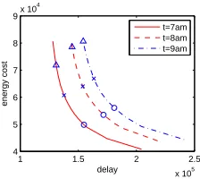
Energy versus delay tradeoff.
1 1.5 2 2.5 x 10⁵ 4
5 6 7 8 9x 10
4
delay
energy cost
t=7am t=8am t=9am
Figure 3: Pareto frontier of the GLB-Q formulation as a function ofβfor three different times (and thus arrival rates), PDT. Circles, x-marks, and triangles correspond toβ= 2.5, 1, and 0.4, respectively.
and energy cost trade off under the optimal solution as β
changes. Thus, the plot shows the Pareto frontier for the GLB-Q formulation. The figure highlights that there is a smooth convex frontier with a mild ‘knee’.
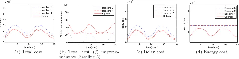
Cost savings.
To evaluate the cost savings of geographical load balanc-ing, Figure 4 compares the optimal costs to those incurred under the three baseline strategies described in the experi-mental setup. The overall cost, shown in Figures 4(a) and 4(b), is significantly lower under the optimal solution than all of the baselines (nearly 40% during times of light traffic). Recall that Baseline 2 is the state of the art, studied in recent papers such as [32, 34].
To understand where the benefits are coming from, let us consider separately the two components of cost: delay and energy. Figures 4(c) and 4(d) show that the optimal algo-rithm performs well with respect to both delay and energy costs individually. In particular, Baseline 1 provides a lower bound on the achievable delay costs, and the optimal algo-rithm nearly matches this lower bound. Similarly, Baseline 2 provides a natural bar for comparing the achievable energy cost. At periods of light traffic the optimal algorithm pro-vides nearly the same energy cost as this baseline, and (per-haps surprisingly) during periods of heavy-traffic the optimal algorithm provides significantly lower energy costs. The ex-planation for this is that, when network delay is considered by the optimal algorithm, if all the close data centers have all servers active, a proxy might still route to them; how-ever when network delay is not considered, a proxy is more likely to route to a data center that is not yet running at full capacity, thereby adding to the energy cost.
Sensitivity analysis.
Given that the algorithms all rely on estimates of theLj
and dij it is important to perform a sensitivity analysis to
understand the impact of errors in these parameters on the achieved cost. We have performed such a sensitivity analysis but omit the details for brevity. The results show that even when the algorithms have very poor estimates ofdijandLj
there is little effect on cost. Baseline 2 can be thought of as applying the optimal algorithm to very poor estimates of
dij (namelydij= 0), and so the Figure 4(a) provides some
illustration of the effect of estimation error.
6.
SOCIAL IMPACT
We now shift focus from the cost savings of the data center operator to the social impact of geographical load balancing. We focus on the impact of geographical load balancing on the usage of “brown” non-renewable energy by Internet-scale systems, and how this impact depends on pricing.
Intuitively, geographical load balancing allows the traffic
to “follow the renewables”; thus providing increased usage of green energy and decreased brown energy usage. However, such benefits are only possible if data centers forgo static energy contracts for dynamic energy pricing (either through demand-response programs or real-time markets). The ex-periments in this section show that if dynamic pricing is done optimally, then geographical load balancing can provide sig-nificant social benefits.
6.1
Experimental setup
To explore the social impact of geographical load balanc-ing, we use the setup described in Section 5. However, we add models for the availability of renewable energy, the pric-ing of renewable energy, and the social objective.
The availability of renewable energy.
To model the availability of renewable energy we use stan-dard models of wind and solar from [15, 20]. Though simple, these models capture the average trends for both wind and solar accurately. Since these models are smoother than ac-tual intermittent renewable sources, especially wind, they conservatively estimate the benefit due to following renew-ables.
We consider two settings (i) high wind penetration, where 90% of renewable energy comes from wind and (ii) high so-lar penetration, where 90% of renewable energy comes from solar. The availability given by these models is shown in Figure 5(a). Setting (i) is motivated by studies such as [18]. Setting (ii) is motivated by the possibility of on-site or locally contracted solar, which is increasingly common.
Building on these availability models, for each location we letαi(t) denote the fraction of the energy that is from
renew-able sources at timet, and let ¯α= (|N|T)−1PT
t=1 P
i∈Nαi(t)
be the “penetration” of renewable energy. We take ¯α= 0.30, which is on the progressive side of the renewable targets among US states [10].
Finally, when measuring the brown/green energy usage of a data center at timet, we use simplyP
i∈Nαi(t)mi(t) as the
green energy usage andP
i∈N(1−αi(t))mi(t) as the brown
energy usage. This models the fact that the grid cannot differentiate the source of the electricity provided.
Demand response and dynamic pricing.
Internet-scale systems have flexibility in energy usage that is not available to traditional energy consumers; thus they are well positioned to take advantage of demand-response and real-time markets to reduce both their energy costs and their brown energy consumption.
To provide a simple model of demand-response, we use time-varying prices pi(t) in each time-slot that depend on
the availability of renewable resourcesαi(t) in each location.
The way pi(t) is chosen as a function of αi(t) will be of
fundamental importance to the social impact of geographical load balancing. To highlight this, we consider a parameter-ized “differentiated pricing” model that uses a price pb for
brown energy and a pricepg for green energy. Specifically,
pi(t) =pb(1−αi(t)) +pgαi(t).
Note that pg =pb corresponds to static pricing, and we
show in the next section thatpg = 0 corresponds to socially
optimal pricing. Our experiments varypg∈[0, pb].
The social objective.
12 24 36 48
% total cost improvement
Baseline 2 Baseline 1 Optimal
(b) Total cost (% improve-ment vs. Baseline 3)
12 24 36 48
Figure 4: Impact of information used on the cost incurred by geographical load balancing.
12 24 36 48
(b) High solar penetration
12 24 36 48
(c) High wind penetration
12 24 36 48
Figure 5: Geographical load balancing “following the renewables” under optimal pricing. (a) Availability of wind and solar. (b)–(d) Capacity provisioning of east coast and west coast data centers when there are renewables, high solar penetration, and high wind penetration, respectively.
purely minimizing brown energy use requires allmi= 0. The
key difference between the GLB formulation and the social formulation is that thecost of energy is no longer relevant. Instead, the environmental impact is important, and thus the brown energy usage should be minimized. This leads to the following simple model for the social objective:
min
cost defined in (1), and ˜β is the relative valuation of delay versus energy. Further, we have imposed that the energy cost follows from the pricing ofpi(t) cents/kWh in timeslot
t. Note that, though simple, our choice ofDi(t) to model the
disutility of delay to users is reasonable because lost revenue captures the lack of use as a function of increased delay.
An immediate observation about the above social objective is that to align the data center and social goals, one needs to setpi(t) = (1−αi(t))/β˜, which corresponds to choosing
pb = 1/β˜ and pg = 0 in the differentiated pricing model
above. We refer to this as the “optimal” pricing model.
6.2
The importance of dynamic pricing
To begin our experiments, we illustrate that optimal pric-ing can lead geographical load balancpric-ing to “follow the re-newables.” Figure 5 shows this in the case of high solar penetration and high wind penetration for ˜β = 0.1. By comparing Figures 5(b) and 5(c) to Figure 5(d), which uses static pricing, the change in capacity provisioning, and thus energy usage, is evident. For example, Figure 5(b) shows a clear shift of service capacity from the east coast to the west coast as solar energy becomes highly available and then
20 40 60 80 100 0
5 10 15
weight for brown energy usage
% social cost improvement
pg=0 pg=0.25 pb pg=0.50pb pg=0.75pb
(a) High solar penetration
20 40 60 80 100
weight for brown energy usage
% social cost improvement
p
(b) High wind penetration
Figure 6: Reduction in social cost from dynamic pricing compared to static pricing as a function of the weight for brown energy usage, 1/β˜, under (a) high solar penetration and (b) high wind penetra-tion.
back when solar energy is less available. Similarly, Figure 5(c) shows a shift, though much smaller, of service capacity toward the evenings, when wind is more available. Though not explicit in the figures, this “follow the renewables” rout-ing has the benefit of significantly reducrout-ing the brown energy usage since energy use is more correlated with the availabil-ity of renewables. Thus, geographical load balancing pro-vides the opportunity to aid the incorporation of renewables into the grid.
Figure 6 focuses on this issue. To model the partial adop-tion of dynamic pricing, we can considerpg ∈[0, pb]. Figure
6(a) shows that the benefits provided by dynamic pricing are moderate but significant, even at partial adoption (highpg),
when there is high solar penetration. Figure 6(b) suggests that there would be much less benefit if renewable sources were dominated by wind with only diurnal variation, because the availability of solar energy is much more correlated with the traffic peaks. Specifically, the three hour gap in time zones means that solar on the west coast can still help with the high traffic period of the east coast, but the peak average wind energy is at night. However, wind is vastly more bursty than this model predicts, and a system which responds to these bursts will still benefit significantly.
Another interesting observation about the Figure 6 is that the curves increase faster in the range when ˜βis large, which highlights that the social benefit of geographical load bal-ancing becomes significant even when there is only moder-ate importance placed on energy. Whenpgis higher thanpb,
which is common currently, the cost increases, but we omit the results due to space constraints.
7.
CONCLUDING REMARKS
This paper has focused on understanding algorithms for and social impacts of geographical load balancing in Internet-scaled systems. We have provided two distributed algorithms that provably compute the optimal routing and provision-ing decisions for Internet-scale systems and we have eval-uated these algorithms using trace-based numerical simula-tions. Further, we have studied the feasibility and benefits of providing demand response for the grid via geographical load balancing. Our experiments highlight that geographical load balancing can provide an effective tool for demand-response: when pricing is done carefully electricity providers can mo-tivate Internet-scale systems to “follow the renewables” and route to areas where green energy is available. This both eases the incorporation of renewables into the grid and re-duces brown energy consumption of Internet-scale systems.
There are a number of interesting directions for future work that are motivated by the studies in this paper. With respect to the design of distributed algorithms, one aspect that our model has ignored is the switching cost (in terms of delay and wear-and-tear) associated with switching servers into and out of power-saving modes. Our model also ignores issues related to reliability and availability, which are quite important in practice. With respect to the social impact of geographical load balancing, our results highlight the oppor-tunity provided by geographical load balancing for demand response; however there are many issues left to be consid-ered. For example, which demand response market should Internet-scale systems participate in to minimize costs? How can policy decisions such as cap-and-trade be used to pro-vide the proper incentives for Internet-scale systems, such as [23]? Can Internet-scale systems use energy storage at data centers in order to magnify cost reductions when participat-ing in demand response markets? Answerparticipat-ing these questions will pave the way for greener geographic load balancing.
8.
ACKNOWLEDGMENTS
This work was supported by NSF grants CCF 0830511, CNS 0911041, and CNS 0846025, DoE grant DE-EE0002890, ARO MURI grant W911NF-08-1-0233, Microsoft Research, Bell Labs, the Lee Center for Advanced Networking, and ARC grant FT0991594.
9.
REFERENCES
[1] US Census Bureau, http://www.census.gov.
[2] Server and data center energy efficiency, Final Report to Congress, U.S. Environmental Protection Agency, 2007. [3] V. K. Adhikari, S. Jain, and Z.-L. Zhang. YouTube traffic
dynamics and its interplay with a tier-1 ISP: An ISP perspective. InACM IMC, pages 431–443, 2010.
[4] S. Albers. Energy-efficient algorithms.Comm. of the ACM, 53(5):86–96, 2010.
[5] L. L. H. Andrew, M. Lin, and A. Wierman. Optimality, fairness and robustness in speed scaling designs. InProc. ACM Sigmetrics, 2010.
[6] A. Beloglazov, R. Buyya, Y. C. Lee, and A. Zomaya. A taxonomy and survey of energy-efficient data centers and cloud computing systems, Technical Report, 2010.
[7] D. P. Bertsekas.Nonlinear Programming. Athena Scientific, 1999.
[8] D. P. Bertsekas and J. N. Tsitsiklis.Parallel and Distributed Computation: Numerical Methods. Athena Scientific, 1989. [9] S. Boyd and L. Vandenberghe.Convex Optimization.
Cambridge University Press, 2004.
[10] S. Carley. State renewable energy electricity policies: An empirical evaluation of effectiveness.Energy Policy, 37(8):3071–3081, Aug 2009.
[11] Y. Chen, A. Das, W. Qin, A. Sivasubramaniam, Q. Wang, and N. Gautam. Managing server energy and operational costs in hosting centers. InProc. ACM Sigmetrics, 2005. [12] M. Conti and C. Nazionale. Load distribution among
replicated web servers: A QoS-based approach. InProc. ACM Worksh. Internet Server Performance, 1999. [13] A. Croll and S. Power. How web speed affects online
business KPIs. http://www.watchingwebsites.com, 2009. [14] X. Fan, W.-D. Weber, and L. A. Barroso. Power
provisioning for a warehouse-sized computer. InProc. Int. Symp. Comp. Arch., 2007.
[15] M. Fripp and R. H. Wiser. Effects of temporal wind patterns on the value of wind-generated electricity in california and the northwest.IEEE Trans. Power Systems, 23(2):477–485, May 2008.
[16] A. Gandhi, M. Harchol-Balter, R. Das, and C. Lefurgy. Optimal power allocation in server farms. InProc. ACM Sigmetrics, 2009.
[17] http://www.datacenterknowledge.com, 2008. [18] http://www.eia.doe.gov.
[19] S. Irani and K. R. Pruhs. Algorithmic problems in power management.SIGACT News, 36(2):63–76, 2005.
[20] T. A. Kattakayam, S. Khan, and K. Srinivasan. Diurnal and environmental characterization of solar photovoltaic panels using a PC-AT add on plug in card.Solar Energy Materials and Solar Cells, 44(1):25–36, Oct 1996.
[21] S. Kaxiras and M. Martonosi.Computer Architecture Techniques for Power-Efficiency. Morgan & Claypool, 2008. [22] R. Krishnan, H. V. Madhyastha, S. Srinivasan, S. Jain,
A. Krishnamurthy, T. Anderson, and J. Gao. Moving beyond end-to-end path information to optimize CDN performance. InProc. ACM Sigcomm, 2009.
[23] K. Le, R. Bianchini, T. D. Nguyen, O. Bilgir, and M. Martonosi. Capping the brown energy consumption of internet services at low cost. InProc. IGCC, 2010. [24] M. Lin, A. Wierman, L. L. H. Andrew, and E. Thereska.
Dynamic right-sizing for power-proportional data centers. In Proc. IEEE INFOCOM, 2011.
[25] Z. M. Mao, C. D. Cranor, F. Bouglis, M. Rabinovich, O. Spatscheck, and J. Wang. A precise and efficient evaluation of the proximity between web clients and their local DNS servers. InUSENIX, pages 229–242, 2002. [26] E. Ng and H. Zhang. Predicting internet network distance
with coordinates-based approaches. InProc. IEEE INFOCOM, 2002.
[27] S. Ong, P. Denholm, and E. Doris. The impacts of commercial electric utility rate structure elements on the economics of photovoltaic systems. Technical Report NREL/TP-6A2-46782, National Renewable Energy Laboratory, 2010.
S. Seshan. On the responsiveness of DNS-based network control. InProc. IMC, 2004.
[30] M. Pathan, C. Vecchiola, and R. Buyya. Load and proximity aware request-redirection for dynamic load distribution in peering CDNs. InProc. OTM, 2008. [31] A. Qureshi, R. Weber, H. Balakrishnan, J. Guttag, and
B. Maggs. Cutting the electric bill for internet-scale systems. InProc. ACM Sigcomm, Aug. 2009.
[32] L. Rao, X. Liu, L. Xie, and W. Liu. Minimizing electricity cost: Optimization of distributed internet data centers in a multi-electricity-market environment. InINFOCOM, 2010. [33] R. T. Rockafellar.Convex Analysis. Princeton University
Press, 1970.
[34] R. Stanojevic and R. Shorten. Distributed dynamic speed scaling. InProc. IEEE INFOCOM, 2010.
[35] W. Theilmann and K. Rothermel. Dynamic distance maps of the internet. InProc. IEEE INFOCOM, 2001.
[36] E. Thereska, A. Donnelly, and D. Narayanan. Sierra: a power-proportional, distributed storage system. Technical Report MSR-TR-2009-153, Microsoft Research, 2009. [37] O. S. Unsal and I. Koren. System-level power-aware deisgn
techniques in real-time systems.Proc. IEEE, 91(7):1055–1069, 2003.
[38] R. Urgaonkar, U. C. Kozat, K. Igarashi, and M. J. Neely. Dynamic resource allocation and power management in virtualized data centers. InIEEE NOMS, Apr. 2010. [39] P. Wendell, J. W. Jiang, M. J. Freedman, and J. Rexford.
Donar: decentralized server selection for cloud services. In Proc. ACM Sigcomm, pages 231–242, 2010.
[40] A. Wierman, L. L. H. Andrew, and A. Tang. Power-aware speed scaling in processor sharing systems. InProc. IEEE INFOCOM, 2009.
APPENDIX
A.
PROOFS FOR SECTION 3
We now prove the results from Section 3, beginning with the illuminating Karush-Kuhn-Tucker (KKT) conditions.
A.1
Optimality conditions
As GLB-Q is convex and satisfies Slater’s condition, the KKT conditions are necessary and sufficient for optimal-ity [9]; for the other models they are merely necessary.
GLB-Q:Letωi ≥0 and ¯ωi ≥0 be Lagrange multipliers
corresponding to (4d), andδij ≥0, νj and σi be those for
(4c), (4b) and (6b). The Lagrangian is then
L=X
The KKT conditions of stationarity, primal and dual feasi-bility and complementary slackness are:
β
The conditions (19)–(22) determine the sources’ choice of
λij, and we claim they imply that source j will only send
data to those data centersiwhich have minimum marginal costdij+ (1 +
i. Thus, from (19), at the optimal point,
dij+
with equality ifλij>0 by (20), establishing the claim.
Note that the solution to (19)–(22) for sourcej depends onλik, k 6= j, only through mi. Given λi, data center i
findsmi as the projection onto [0, Mi] of the solution ˆmi=
λi(1 +ppi/β)/(µippi/β) of (23) with ¯ωi=ωi= 0.
GLB-LIN again decouples into data centers finding mi
given λi, and sources finding λij given the mi.
Feasibil-ity and complementary slackness conditions (20), (22), (24) and (25) are as for GLB-Q; the stationarity conditions are:
∂gi(mi, λi)
Note the feasibility constraint (6b) of GLB-Q is no longer re-quired to ensure stability. In GLB-LIN, it is instead assumed thatf is infinite when the load exceeds capacity.
The objective function is strictly convex in data centeri’s decision variablemi, and so there is a unique solution ˆmi(λi)
to (28) for ¯ωi=ωi = 0, and the optimalmigiven λiis the
projection of this onto the interval [0, Mi].
GLBin its general form has the same KKT conditions as GLB-LIN, with the stationary conditions replaced by
∂gi
GLB again decouples, since it is convex because r(·) is convex and increasing. However, now data centeri’s problem depends on allλij, rather than simplyλi.
A.2
Characterizing the optima
Lemma 7 will help prove the results of Section 3.
Lemma 7. Consider the GLB-LIN formulation. Suppose that for all i, Fi(mi, λi) is jointly convex inλi andmi, and
differentiable inλi where it is finite. If, for somei, the dual
variable ω¯i >0for an optimal solution, then mi =Mi for
all optimal solutions. Conversely, ifmi< Mi for an optimal
solution, then ω¯i= 0for all optimal solutions.
Proof. Consider an optimal solutionS withi∈N such
that ¯ωi > 0 and hence mi = Mi. Let S′ be some other
optimal solution.
Since the cost function is jointly convex in λij and mi,
any convex combination of S and S′ must also be optimal.
Let mi(s) denote themi value of a given solution s. Since
mi(S) = Mi, we have λi > 0 and so the optimality of S
impliesfiis finite atSand hence differentiable. By (28) and
SinceS+ǫ(S′−S)∈ N for sufficiently smallǫ, the linearity of mi(s) impliesMi=mi(S+ǫ(S′−S)) =mi(S) +ǫ(mi(S′)−
mi(S)). Thusmi(S′) =mi(S) =Mi.
Proof of Theorem 1. Consider first the case where there
exists an optimal solution with mi < Mi. By Lemma 7,
¯
ωi = 0 for all optimal solutions. Recall that ˆmi(λi), which
defines the optimalmi, is strictly convex. Thus, if different
optimal solutions have different values of λi, then a
con-vex combination of the two yielding (m′
i, λ′i) would have
ˆ
mi(λ′i)< m′i, which contradicts the optimality ofm′i.
Next consider the case where all optimal solutions have
mi=Mi. In this case, consider two solutionsS andS′ that
both havemi=Mi. Ifλiis the same under bothS andS′,
we are done. Otherwise, let the set of convex combinations of
S and S′ be denoted{s(λi)}, where we have made explicit
the parameterization by λi. The convexity of each Fk in
mkandλk implies thatF(s(λi))−Fi(s(λi)) is also convex,
due to the fact that the parameterization is by definition affine. Further, sinceFiis strictly convex inλi, this implies
F(s(λi)) is strictly convex in λi, and hence has a unique
optimalλi.
Proof of Theorem 2. The proof whenmi=Mifor all
optimal solutions is identical to that of Theorem 1. Other-wise, when mi < Mi in an optimal solution, the definition
of ˆmgivesλi=µippi/βi/(ppi/βi+ 1) for all optimal
solu-tions.
Proof of Theorem 3. For each optimal solutionS,
con-sider an undirected bipartite graphG with a vertex repre-senting each source and each data center and with an edge connectingiandjwhenλij>0. We will show that at least
one of these graphs is acyclic. The theorem then follows since an acyclic graph withK nodes has at mostK−1 edges.
To prove that there exists one optimal solution with acyclic graph we will inductively reroute traffic in a way that re-moves cycles while preserving optimality. Suppose G con-tains a cycle. LetCbe a minimal cycle, i.e., no strict subset ofC is a cycle, and letCbe directed.
Form a new solution S(ξ) from S by adding ξ to λij if
(i, j)∈C, and subtractingξfromλijif (j, i)∈C. Note that
this does not change theλi. To see that S(ξ) is maintains
the optimal cost, first note that the change in the objective function of the GLB betweenS andS(ξ) is equal to
ξ
X
(j,i)∈C
r(dij+fi(mi, λi))−
X
(i,j)∈C
r(dij+fi(mi, λi))
(31)
Next note that the multiplier δij = 0 since λij > 0 at S.
Further, the KKT condition (29) for stationarity inλijcan
be written asKi+r(dij+fi(mi, λi))−νj = 0,where Ki
does not depend on the choice ofj.
SinceC is minimal, for each (i, j) ∈C where i∈ I and
j∈J there is exactly one (j′, i) withj′∈J, and vice versa.
Thus,
0 =X
(j,i)∈C
(Ki+r(dij+fi(mi, λi))−νj)
−X
(i,j)∈C
(Ki+r(dij+fi(mi, λi))−νj)
=X
(j,i)∈C
r(dij+fi(mi, λi))−
X
(i,j)∈C
r(dij+fi(mi, λi)).
Hence, by (31) the objective ofS(ξ) andS are the same. To complete the proof, we let (i∗, j∗) = arg min(i,j)∈Cλij.
ThenS(λi∗,j∗) hasλi∗,j∗ = 0. Thus,S(λi∗,j∗) has at least
one fewer cycle, since it has brokenC. Further, by construc-tion, it is still optimal.
Proof of Theorem 4. It is sufficient to show that, if λkjλk′j>0 then eithermk=Mk ormk′ =Mk′. Consider
a case whenλkjλk′j>0.
For a generici, defineci= (1 +
p
pi/β)2/µias the marginal
cost (26) when the Lagrange multipliers ¯ωi=ωi= 0. Since
the pi are chosen from a continuous distribution, we have
that with probability 1
ck−ck′ 6=dk′j−dkj. (32)
However, (26) holds with equality ifλij>0, and sodkj+
(1 +p
p∗
k/β)2/µk=dk′j+ (1 +
p
p∗
k′/β)
2/µ
k′. By the
defi-nition ofciand (32), this implies eitherp∗k6=pkorp∗k′ 6=pk.
Hence at least one of the Lagrange multipliersωk, ¯ωk,ωk′ or
¯
ωk′ must be non-zero. However,ωi>0 would implymi= 0
whenceλij= 0 by (21), which is false by hypothesis, and so
either ¯ωk or ¯ωk′ is non-zero, giving the result by (24).
B.
PROOFS FOR SECTION 4
Algorithm 1
To prove Theorem 5 we apply a variant of Proposition 3.9 of Ch 3 in [8], which gives that if
(i) F(m,λ) is continuously differentiable and convex in the
convex feasible region (4b)–(4d);
(ii) Every limit point of the sequence is feasible;
(iii) Given the values ofλ−j andm, there is a unique
min-imizer of F with respect toλj, and given λthere is a
unique minimizer ofF with respect tom.
Then, every limit point of (m(τ),λ(τ))τ=1,2,...is an optimal
solution of GLB-Q.
This differs slightly from [8] in that the requirement that the feasible region be closed is replaced by the feasibility of all limit points, and the requirement of strict convexity with respect to each component is replaced by the existence of a unique minimizer. However, the proof is unchanged.
Proof of Theorem 5. To apply the above to prove
The-orem 5, we need to show thatF(m,λ) satisfies the
differen-tiability and continuity constraints under the GLB-Q model. GLB-Q is continuously differentiable and, as noted in Ap-pendix A.1, a convex problem. To see that every limit point is feasible, note that the only infeasible points in the clo-sure of the feasible region are those withmiµi =λi. Since
the objective approaches∞approaching that boundary, and Gauss-Seidel iterations always reduce the objective [8], these points cannot be limit points.
It remains to show the uniqueness of the minimum in m
and each λj. Since the cost is separable in the mi, it is
sufficient to show that this applies with respect to eachmi
individually. Ifλi= 0, then the unique minimizer ismi= 0.
Otherwise
∂2F(m,λ)
∂m2
i
= 2βµi λ
2
i
(miµi−λi)3
which by (6b) is strictly positive. The Hessian of F(m,λ)
with respect toλj is diagonal withith element
2βµi m
2
i
(miµi−λi)3
>0
which is positive definite except the points where somemi=
0. However, ifmi= 0, the unique minimum isλij= 0. Note
we cannot have all mi = 0. Except these points, F(m,λ)
is strictly convex in λj given m andλ−j. Therefore λj is
Part (ii) of Theorem 5 follows from part (i) and the con-tinuity ofF(m,λ). Part (iii) follows from part (i) and
The-orem 2, which provides the uniqueness of optimal per-server arrival rates (λi(τ)/mi(τ), i∈N).
Algorithm 2
As discussed in the section on Algorithm 2, we will prove Theorem 6 in three steps. First, we will show that, starting from an initial feasible point λ(0), Algorithm 2 generates
a sequence λ(τ) that lies in the set Λ := Λ(φ) defined in
(15), for τ = 0,1, . . .. Moreover, ∇F(λ) is Lipschitz over
Λ. Finally, this implies that F(λ(τ)) moves in a descent
direction that guarantees convergence.
Lemma 8. Given an initial pointλ(0)∈Q
the following intermediate result. We omit the proof due to space constraint.
Proof. Following Lemma 9, here we continue to show
∞. The inequality is a property of norms and
the equality is from the symmetry of∇2F(M,λ). Finally,
Lemma 11. When applying Algorithm 2 to GLB-Q, (a)F(λ(τ+1))≤F(λ(τ))−( 1
Proof. From the Lemma 10, we know
the property of gradient projection. The last line is from the definition of γm.
each gradient projection, we know it is optimal. Conversely, ifλ(τ) minimizesF(λ(τ)) over the set Λ, then the gradient
projection always projects to the original point, henceZj(τ+ 1) =λj(τ),∀j. See also [8, Ch 3 Prop. 3.3(b)] for reference.
(c) SinceF(λ) is continuously differentiable, the gradient
mapping is continuous. The projection mapping is also con-tinuous. T is the composition of the two and is therefore continuous.
Proof of Theorem 6. Lemma 11 is parallel to that of