Geographical Load Balancing with Renewables
∗Zhenhua Liu, Minghong Lin,
Adam Wierman, Steven H. Low
CMS, California Institute of Technology, Pasadena{zliu2,mhlin,adamw,slow}@caltech.edu
Lachlan L. H. Andrew
Faculty of ICTSwinburne University of Technology, Australia
[email protected]
ABSTRACT
Given the significant energy consumption of data centers, im-proving their energy efficiency is an important social prob-lem. However, energy efficiency is necessary but not suf-ficient for sustainability, which demands reduced usage of energy from fossil fuels. This paper investigates the feasi-bility of powering internet-scale systems using (nearly) en-tirely renewable energy. We perform a trace-based study to evaluate three issues related to achieving this goal: the impact of geographical load balancing, the role of storage, and the optimal mix of renewables. Our results highlight that geographical load balancing can significantly reduce the required capacity of renewable energy by using the energy more efficiently with “follow the renewables” routing. Fur-ther, our results show that small-scale storage can be useful, especially in combination with geographical load balancing, and that an optimal mix of renewables includes significantly more wind than photovoltaic solar.
1.
INTRODUCTION
Energy consumption of data centers is of growing concern to both operators and society. Electricity for internet-scale systems costs millions of dollars per month [16] and, though ICT uses only a small percentage of electricity today, the growth of electricity in ICT exceeds nearly all sectors of the economy. For these reasons, and more, ICT must play its part in reducing our dependence on fossil fuels.
This can be achieved by using renewable energy to power data centers. Already, data centers are often powered by a “green” portfolio of energy [8, 11, 13]. However, most stud-ies of powering data centersentirelywith renewable energy have focused on powering individual data centers, e.g., [3, 4]. These have shown that it is challenging to power a data center using only local wind and solar energy without large-scale storage, due to the intermittency and unpredictability of these sources
The goal of this paper is to illustrate that the geographical diversity of internet-scale services significantly improves the efficiency of the usage of renewable energy. This numerical
∗This work was supported by NSF grants CCF 0830511, CNS 0911041, and CNS 0846025, DoE grant DE-EE0002890, ARO MURI grant W911NF-08-1-0233, Microsoft Research, Bell Labs, the Lee Center for Advanced Networking, and ARC grant FT0991594.
Permission to make digital or hard copies of all or part of this work for personal or classroom use is granted without fee provided that copies are not made or distributed for profit or commercial advantage and that copies bear this notice and the full citation on the first page. To copy otherwise, to republish, to post on servers or to redistribute to lists, requires prior specific permission and/or a fee.
Copyright 200X ACM X-XXXXX-XX-X/XX/XX ...$10.00.
study complements testbeds such [15]. Further, we illustrate that algorithmic solutions, such as geographical load balanc-ing (GLB), can play a vital role in reducbalanc-ing the necessary capacity of renewable energy installed.
Specifically, we perform numerical experiments using real traffic workloads and real data about the availability of re-newables combined with an analytic model for a geograph-ically distributed system. Using this setup, we investigate issues related to the feasibility of powering an internet-scale system (nearly) completely with renewable energy.
Our study yields three key insights.
First, GLB significantly reduces the capacity of renewables needed to move toward a “green” system, since GLB allows the system to use “follow the renewables” routing, which re-duces both the financial cost and the “brown” non-renewable energy usage. However, we also show the importance of us-ing a fast control time-scale for GLB. If routus-ing and capacity decisions are made only once an hour, then significantly more brown energy is consumed than if the adjustments are made every ten minutes. Unfortunately, adjustments at this faster time-scale may not be feasible due to server wear-and-tear and other concerns.
Second, we investigate the value of storage when using re-newable energy. Often large-scale storage is viewed as essen-tial for moving toward a completely renewable energy port-folio. However, our study shows that small-scale storage in combination with GLB is sufficient in moving to a portfo-lio of nearly completely renewable energy sources. This is particularly exciting since the UPSs in use at data centers today could be used to provide small-scale storage with few engineering changes.
Third, we find that wind is more valuable than solar for internet-scale systems, especially when GLB is used, because wind has little correlation across locations, and is available during both night and day. Thus, if one aggregates over many locations, there is much less variation in the availabil-ity [2]. The optimal mix seems to be dominated by wind, but include some solar to handle the peak workload around noon. For the traces we consider, the optimal portfolio is 80% wind and 20% solar. This ratio may depend on the quality of the local wind resources; moreover, workloads with higher (lower) diurnal peak-to-mean ratios may benefit from a higher (lower) solar component.
2.
SETUP
Our numeric experiments combine analytic models with real traces for workload and renewable availability, to allow controlled experimentation but provide realistic findings. We now explain the setup, which extends that of [10].
2.1
The workload
conti-0 24 48 72 96 120 144 168 0
2 4 6 8
hour
workload
(a) One week workload
0 6 12 18 24
0 2 4 6 8
hour
workload
(b) Tuesday workload
Figure 1: HP workload trace.
nental states in the US.
We consider one hour time slots for a week. At the start of each slot, the routing and capacity of each data center are updated. We use a slot length of 1 hour so that servers are not turned on and off too frequently given the significant wear-and-tear costs of power-cycling. LetLj(t) denote the mean arrival rate from sourcejat timet.
To provide realistic estimates, we use real-world traces to defineLj(t). The workload of each source is scaled propor-tionally to the number of internet users in the corresponding state. The workload is taken from a trace at Hewlett-Packard Labs [4] and is shifted in time to account for time zone of each state. The workload per internet user used in this paper is shown in Figure 1.
2.2
The availability of renewable energy
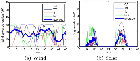
To capture the availability of wind and solar energy, we use traces of wind speed and Global Horizontal Irradiance obtained from [5, 6] that have measurements every 10 min-utes for a year. The traces of four states (CA, TX, IL, NC) are illustrated in Figure 2. Note that as “solar”,we only con-sider photovoltaic generation and not solar thermal, because of the significant infrastructure required for solar thermal plants. Since solar thermal plants typically incorporate a day’s thermal storage [14], the results would be very differ-ent if solar thermal were considered. Also, note that the wind and solar capacities are calculated as the amount achievable by a 30 kW wind turbine and 4 kW photovoltaic panel.
These figures illustrate two important features of renew-able energy: spatial variation and temporal variation. In particular, we see that wind energy does not exhibit a clearly predictable pattern throughout the day and that there is lit-tle correlation across the locations considered. In contrast, solar energy has a predictable peak during the day and is highly correlated across the locations.
In our investigation, we scale the “capacity” of wind and solar. When doing so, we scale the availability of wind and solar linearly, which is suitable when considering scaling the size of the wind farm or solar installation. Throughout, we measure the capacity of renewables as the ratio of the average renewable generation to the minimal energy required to serve the average workload. Thus, a capacity ofc= 2 means that the average renewable generation is twice the minimal energy required to serve the average workload. In the following we set capacity toc= 2 by default, but vary it in Figures 5–7.
2.3
The internet-scale system
We model the internet-scale system as a setN of 10 data centers, placed at the centers of states known to have Google data centers [12], namely California, Washington, Oregon, Illinois, Georgia, Virginia, Texas, Florida, North Carolina, and South Carolina. Data center i ∈ N contains Mi ho-mogeneous servers, whereMi is twice the minimal number of servers required to serve the peak workload ofiunder a scheme which routes traffic to the nearest data center.
Fur-0 6 12 18 24 30 36 42 48 0
10 20 30 40 50 60
hour
wind power generation (kW)
CA TX IL NC average
(a) Wind
0 6 12 18 24 30 36 42 48
0 1 2 3 4 5
hour
PV generation (kW)
CA TX IL NC average
(b) Solar
Figure 2: Renewable generation for two days.
ther, the renewable availability at each data center is defined by the trace from a nearby location; this was usually within the same state, but in five cases it was a different trace from a nearby state.
The two key control decisions of geographical load balanc-ing are (i) determinbalanc-ing λij(t), the amount of traffic routed from sourcejto data centeri; and (ii) determiningmi(t)∈ {0, . . . , Mi}, the number of active servers at data centeri. The objective is to chooseλij(t) and mi(t) to minimize the “cost” of the system. The cost is the sum of theenergy cost
and thedelay cost(lost revenue), below. We neglect the cost of altering the number of active servers mi(t); this can be incorporated using an approach similar to that of [9].
Delay cost.
The delay cost captures the lost revenue incurred because of the delay experienced by the requests, where the delay includes both the network delay from source jto data cen-teri,dij, and the queueing delay ati. We modeldij to be the distance between source and data center, divided by the speed of 200 km/ms plus a constant (5 ms), resulting in de-lay ranging in [5 ms, 56 ms]. We model the queueing dede-lays using parallel M/G/1/Processor Sharing queues with the to-tal loadλi(t) =Pjλij(t) divided equally among themi(t) active servers, each having service rateµi= 0.1(ms)−1. This parameter setting makes the average delay 20 ms when the utilization is 0.5, which is reasonable. Note that this model is not new, and is referred to as the GLB-LIN-Q model in [10].
Energy cost.
To capture the effect of integrating renewable energy, we model the energy cost as the number of active servers exclud-ing those that can be powered by renewables. Note that this assumes that data centers operate their own wind and solar generations and pay no marginal cost for renewable energy. Further, it ignores the installation and maintenance costs of renewable generation.
Quantitatively, if the renewable energy available at data center iat timet is ri(t), measured in terms of number of servers that can be powered, then the energy cost is
pi(mi(t)−ri(t))+ (1)
Thepi for each data center is constant, and proportional to the industrial electricity price of each state in May 2010 [7]. This contrasts with the total powerpimiused typically, e.g., in [10].
Storage.
0 10 20 30 40
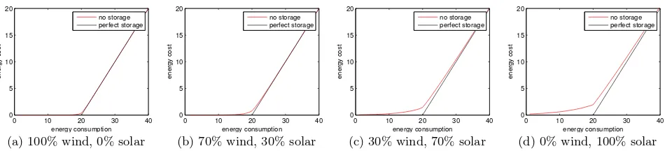
Figure 3: Energy cost as a function of total energy consumption, when the average renewable energy in a one-hour slot is 20.
Without storage, there will be some cost incurred due to the variability of renewable availability within a time slot. Here the actually energy cost becomes
Eτ
ri(t). Figure 3 shows two curves for California. The lower curve corresponds to (1), i.e., the price curve for a system with small-scale storage (which is used to “perfectly” smooth renewable generation) and the upper one for (2), i.e. the case of no storage, which is derived directly from the renew-able traces as described above. The figure illustrates the two curves in the case of an average renewable generation of 20 kW withpi = 1,τ = 10 min, and includes different mix-tures of solar and wind. Interestingly, the added cost for not having storage increases as the percentage of solar increases in the renewable portfolio.
Total cost.
Combining the discussions above, we can now write the total cost for an internet-scale system. In particular, for the case where the data centers have small-scale storage, the cost optimization that system seeks to solve at timetbecomes:
min
Hereβ determines the relative importance of energy and delay to the system. In the simulations β is set to 1 by default, but we also varyβ∈[1,10] in Figure 4 to show its impact. This range corresponds to a realistic cost of latency, e.g., see [1].
When data centers have no energy storage, only the energy cost component of the optimization changes from (1) to (2). However, we cannot write the optimization in closed form for that case because the energy cost curves are determined by the renewable energy traces, as shown in Figure 3. To formulate and solve the optimization in this case we use a piecewise-linear approximation of the curves in Figure 3.
Geographical load balancing.
The above sections describe the cost optimization that the internet-scale system seeks to solve; however they do not de-scribe how the system actually performs geographical load balancing to solve the optimization. In [10], decentralized algorithms are presented, which can be used to achieve the optimal cost in the setting described above. Thus, in this paper we present as “GLB” the routing and capacity provi-sioning decisions which solve the cost optimization problem. Note that the results do not rely on the algorithms in [10]; they simply consider the optimal allocation.
As a benchmark for comparison, we consider a system that does no geographical load balancing, but instead routes all requests to the nearest data center and optimally adjusts the number of active servers at each location. We call this system ‘LOCAL’ and use it to illustrate the benefits that come from using geographical load balancing.
3.
RESULTS
With the setup described in the previous section, we have performed a number of numerical experiments to evaluate the feasibility of moving toward internet-scale systems pow-ered (nearly) entirely by renewable energy. We focus on three issues: (i) the impact of geographical load balancing, (ii) the role of storage, and (iii) the optimal mix of wind and solar.
3.1
The impact of geographical load balancing
Geographical load balancing is known to provide internet-scale system operators significant energy cost savings, at the expense of small increases in network delay due to the fact that requests can be routed to where energy is cheap or re-newable generation is high. This behavior is illustrated in Figure 4, which shows the average cost and delay under GLB versus LOCAL as the cost (β) of brown energy relative to delay is increased. The novelty of Figure 4 is in (a), which shows the reduction in consumption of brown energy. This illustrates that the reduction in brown consumption is sig-nificantly larger even than the reduction in cost, and that it is significant even when energy is cheap (βis small).
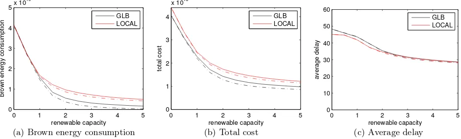
Next, we consider Figure 5, which illustrates the differ-ences between LOCAL and GLB as a function of the capac-ity of renewable energy. Interestingly, Figure 5 highlights that when there is little capacity of renewables, both GLB and LOCAL can take advantage of it, but that as the ca-pacity of renewables increases GLB is much more efficient at using it. This is evident because of the significantly lower brown energy consumption of GLB that emerges at capac-ities>1.5. Figure 5 also illustrates that increased capacity provides significant reductions in both the total cost and the average delay under both GLB and LOCAL.
1 2 3 4 5 6 7 8 9 10 0
0.5 1 1.5 2 2.5x 10
10
β
brown energy consumption
GLB LOCAL
(a) Brown energy consumption
1 2 3 4 5 6 7 8 9 10 0
0.5 1 1.5 2 2.5 3
x 1013
β
total cost
GLB LOCAL
(b) Total cost
1 2 3 4 5 6 7 8 9 10
0 10 20 30 40 50 60
β
average delay
GLB LOCAL
(c) Average delay
Figure 4: Comparison of GLB and LOCAL as a function ofβ. The renewable capacity is 2. The dashed line
is the same setting except with storage.
0 1 2 3 4 5
0 1 2 3 4
5x 10
10
renewable capacity
brown energy consumption
GLB LOCAL
(a) Brown energy consumption
0 1 2 3 4 5
0 1 2 3 4
x 1013
renewable capacity
total cost
GLB LOCAL
(b) Total cost
0 1 2 3 4 5
0 10 20 30 40 50 60
renewable capacity
average delay
GLB LOCAL
(c) Average delay
Figure 5: Comparison of GLB and LOCAL with different renewable capacities andβ= 10. The dashed line
is the same setting except with storage.
energy reduction targets. We see in (a) that, under LOCAL, the capacity of renewables necessary to hit an 85% reduction of brown energy is extreme. However, in (b) we see that the use of GLB can provide significant reductions due to its more efficient use of the renewable capacity. If energy is expensive (β= 10), then the required capacity is nearly viable.
The discussion above highlights that GLB can be extremely useful for the adoption of renewable energy into internet-scale systems. However, there are certainly challenges that remain for the design of GLB. One particularly important challenge is that of adjusting the routing and capacity deci-sions at a fast enough time scale to react to the availability of renewable energy. In particular, the plots we have described so far use a control scale of 1 hour. If this control time-scale is slower, or if information about the availability of re-newable energy is stale, then the benefits provided by GLB degrade. This is illustrated in Figure 6(c). This highlights the importance of reducing the energy and wear-and-tear costs of switching servers into and out of active mode, since it is the magnitude of these costs that most often limits the control time-scale.
3.2
The role of storage
In addition to GLB, another important tool to aid the in-corporation of renewable energy into internet-scale systems is storage, such as Uninterruptible Power Supplies (UPSs). In this paper, we limit our consideration to small-scale stor-age, which is only able to power the data center over the time-scale of a few minutes. We consider small-scale storage due to the opportunity provided by the UPSs already
avail-able in data centers today, and due to the fact that the cost of large scale storage is prohibitive at this point.
Throughout Figures 4, 5, 6(a), 6(b), and 7, the impact of storage can be seen through the difference between the corresponding dashed and solid lines. A few trends that are evident in these plots are the following: (i) storage becomes more valuable with either higher capacities of renewables, i.e., >1.5, or largerβ; and (ii) storage plays a more signif-icant role under GLB than under LOCAL. Both points are clearly illustrated in Figures 4 and 5, and Figure 5 also high-lights that storage allows brown energy consumption to be almost completely eliminated when using GLB.
3.3
The optimal renewable portfolio
We now move to the question of what mix of solar and wind is most effective for internet-scale systems. A priori, it seems that solar may be the most effective, since the peak of solar availability is closely aligned with that of the data center workload. However, the fact that solar is not available during the night is a significant drawback. Also, once GLB is used, it becomes possible to aggregate wind availability across geographical locations. This provides significant ben-efits because wind availability is not correlated across large geographical distances, and so when aggregated, the avail-ability smoothes considerably, as illustrated in Figure 2(b). As a result, it seems that wind should be quite valuable to internet-scale systems.
ex-0 0.2 0.4 0.6 0.8 1 0
2 4 6 8
solar capacity
wind capacity
15% 20% 25% 30%
(a) LOCAL for different brown energy targets
0 0.2 0.4 0.6 0.8 1
0 2 4 6 8
solar capacity
wind capacity
LOCAL GLB β=1 GLB β=10
(b) LOCAL and GLB for 15% brown en-ergy target
0 0.2 0.4 0.6 0.8 1
0 2 4 6 8
solar capacity
wind capacity
3hours 2hours 1hour 10min
(c) GLB with different control time-scales and 15% brown energy target
Figure 6: Wind and solar capacity required to reduce brown energy usage to 15–30% of the baseline, as a function of solar capacity. The dashed line is the same setting except with storage.
0 20 40 60 80 100
1 2 3 4 5x 10
10
% of wind
brown energy consumption
c = 1 c = 2 c = 3
(a) Brown energy consumption
0 20 40 60 80 100
7 8 9 10 11 12
x 1012
% of wind
total cost
c = 1 c = 2 c = 3
(b) Total cost
0 20 40 60 80 100
25 25.5 26 26.5 27
% of wind
average delay
c = 1 c = 2 c = 3
(c) Average delay
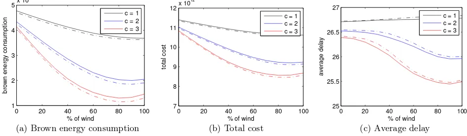
Figure 7: Impact of the mix of renewable energy used under GLB with β = 1 when the total renewable
capacity isc= 1,2,3. The dashed line is the same setting except with storage.
tra solar capacity provides little benefit beyond that point. More specifically, Figure 7 shows the brown energy usage as a function of the fraction of energy coming from wind, for three values of total generating capacity,c. Keepingcfixed implicitly assumes that the cost per kWh of solar and wind installation are equal.
Interestingly, this optimal portfolio is robust to many fac-tors including storage, renewable capacity, and even whether the system seeks to optimize brown energy consumption, to-tal cost, or average delay. This last point is important, since it highlights that the system operators’ goal is aligned with both the users’ experience and society’s interest. However, the optimal portfolio is affected by the workload, specifically, the peak-to-mean ratio. For large diurnal peak-to-mean ra-tios the optimal portfolio can be expected to use a higher percentage of solar.
4.
REFERENCES
[1] The cost of latency.James Hamilton’s Blog, 2009.
[2] C. L. Archer and M. Z. Jacobson. Supplying baseload power and reducing transmission requirements by interconnecting wind farms.J. Applied Meteorology and Climatology, 46:1701–1717, Nov. 2007.
[3] D. Gmach, J. Rolia, C. Bash, Y. Chen, T. Christian, and A. Shah. Capacity planning and power management to exploit sustainable energy. InProc. of CNSM, 2010. [4] D. Gmach, YuanChen, A. Shah, J. Rolia, C. Bash,
T. Christian, and R. Sharma. Profiling sustainability of data centers. InProc. ISSST, 2010.
[5] http://rredc.nrel.gov. 2010.
[6] http://wind.nrel.gov. 2010. [7] http://www.eia.doe.gov. 2010.
[8] M. LaMonica. Google data center to get boost from wind farm.CNET News, 21 April 2011.
[9] M. Lin, A. Wierman, L. L. H. Andrew, and E. Thereska. Dynamic right-sizing for power-proportional data centers. In Proc. of INFOCOM, 2011.
[10] Z. Liu, M. Lin, A. Wierman, S. H. Low, and L. L. H. Andrew. Greening geographic load balancing. InProc. ACM Sigmetrics, 2011.
[11] C. Miller. Solar-powered data centers.Datacenter Knowledge, 13 July 2010.
[12] R. Miller. Google data center FAQ.Datacenter Knowledge, 27 March 2008.
[13] R. Miller. Facebook installs solar panels at new data center. Datacenter Knowledge, 16 April 2011.
[14] D. Mills. Advances in solar thermal electricity technology. solar Energy, 76:19–31, 2004.
[15] K. K. Nguyen, M. Cheriet, M. Lemay, B. St. Arnaud, V. Reijs, A. Mackarel, P. Minoves, A. Pastrama, and W. Van Heddeghem. Renewable energy provisioning for ICT services in a future internet. InFuture Internet Assembly. LNCS 6656, pages 419–429. 2011.