Introduction to Probability Theory and
Statistics
Copyright @ Javier R. Movellan, 2004-2008
Contents
1 Probability 7
1.1 Intuitive Set Theory . . . 10
1.2 Events . . . 14
1.3 Probability measures . . . 14
1.4 Joint Probabilities . . . 16
1.5 Conditional Probabilities . . . 16
1.6 Independence of 2 Events . . . 17
1.7 Independence of n Events . . . 17
1.8 The Chain Rule of Probability . . . 19
1.9 The Law of Total Probability . . . 20
1.10 Bayes’ Theorem . . . 21
1.11 Exercises . . . 22
2 Random variables 25 2.1 Probability mass functions. . . 28
2.2 Probability density functions. . . 30
2.3 Cumulative Distribution Function. . . 32
2.4 Exercises . . . 34
3 Random Vectors 37 3.1 Joint probability mass functions . . . 37
3.2 Joint probability density functions . . . 37
3.3 Joint Cumulative Distribution Functions . . . 38
3.4 Marginalizing . . . 38
3.5 Independence . . . 39
3.6 Bayes’ Rule for continuous data and discrete hypotheses . . . 40
3.6.1 A useful version of the LTP . . . 41
3.7 Random Vectors and Stochastic Processes . . . 42
4 Expected Values 43
4.1 Fundamental Theorem of Expected Values . . . 44
4.2 Properties of Expected Values . . . 46
4.3 Variance . . . 47
4.3.1 Properties of the Variance . . . 48
4.4 Appendix: Using Standard Gaussian Tables . . . 51
4.5 Exercises . . . 52
5 The precision of the arithmetic mean 53 5.1 The sampling distribution of the mean . . . 54
5.1.1 Central Limit Theorem . . . 55
5.2 Exercises . . . 56
6 Introduction to Statistical Hypothesis Testing 59 6.1 The Classic Approach . . . 59
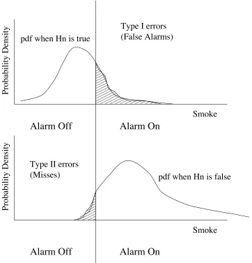
6.2 Type I and Type II errors . . . 61
6.2.1 Specifications of a decision system . . . 63
6.3 The Bayesian approach . . . 63
6.4 Exercises . . . 65
7 Introduction to Classic Statistical Tests 67 7.1 The Z test . . . 67
7.1.1 Two tailed Z test . . . 67
7.1.2 One tailed Z test . . . 69
7.2 Reporting the results of a classical statistical test . . . 71
7.2.1 Interpreting the results of a classical statistical test . . . . 71
7.3 The T-test . . . 72
7.3.1 The distribution of T . . . 73
7.3.2 Two-tailed T-test . . . 74
7.3.3 A note about LinuStats . . . 76
7.4 Exercises . . . 76
7.5 Appendix: The sample variance is an umbiased estimate of the population variance . . . 78
8 Intro to Experimental Design 81 8.1 An example experiment . . . 81
8.2 Independent, Dependent and Intervening Variables . . . 83
CONTENTS 5
8.4 Useful Concepts . . . 87
8.5 Exercises . . . 89
9 Experiments with 2 groups 93 9.1 Between Subjects Experiments . . . 93
9.1.1 Within Subjects Experiments . . . 96
9.2 Exercises . . . 98
10 Factorial Experiments 99 10.1 Experiments with more than 2 groups . . . 99
10.2 Interaction Effects . . . 101
11 Confidence Intervals 103 A Useful Mathematical Facts 107 B Set Theory 115 B.1 Proofs and Logical Truth . . . 118
B.2 The Axioms of Set Theory . . . 119
B.2.1 Axiom of Existence: . . . 119
B.2.2 Axiom of Equality: . . . 120
B.2.3 Axiom of Pair: . . . 120
B.2.4 Axiom of Separation: . . . 121
B.2.5 Axiom of Union: . . . 122
B.2.6 Axiom of Power: . . . 123
B.2.7 Axiom of Infinity: . . . 124
B.2.8 Axiom of Image: . . . 124
B.2.9 Axiom of Foundation: . . . 125
Chapter 1
Probability
Probability theory provides a mathematical foundation to concepts such as “proba-bility”, “information”, “belief”, “uncertainty”, “confidence”, “randomness”, “vari-ability”, “chance” and “risk”. Probability theory is important to empirical sci-entists because it gives them a rational framework to make inferences and test hypotheses based on uncertain empirical data. Probability theory is also useful to engineers building systems that have to operate intelligently in an uncertain world. For example, some of the most successful approaches in machine per-ception (e.g., automatic speech recognition, computer vision) and artificial intel-ligence are based on probabilistic models. Moreover probability theory is also proving very valuable as a theoretical framework for scientists trying to under-stand how the brain works. Many computational neuroscientists think of the brain as a probabilistic computer built with unreliable components, i.e., neurons, and use probability theory as a guiding framework to understand the principles of computation used by the brain. Consider the following examples:
• You need to decide whether a coin is loaded (i.e., whether it tends to favor one side over the other when tossed). You toss the coin 6 times and in all cases you get “Tails”. Would you say that the coin is loaded?
• You are trying tofigure out whether newborn babies can distinguish green from red. To do so you present two colored cards (one green, one red) to 6 newborn babies. You make sure that the 2 cards have equal overall luminance so that they are indistinguishable if recorded by a black and white camera. The 6 babies are randomly divided into two groups. Thefirst group gets the red card on the left visual field, and the second group on the right
visualfield. Youfind that all 6 babies look longer to the red card than the green card. Would you say that babies can distinguish red from green?
• A pregnancy test has a 99 % validity (i.e., 99 of of 100 pregnant women test positive) and 95 % specificity (i.e., 95 out of 100 non pregnant women test negative). A woman believes she has a 10 % chance of being pregnant. She takes the test and tests positive. How should she combine her prior beliefs with the results of the test?
• You need to design a system that detects a sinusoidal tone of 1000Hz in the presence of white noise. How should design the system to solve this task optimally?
• How should the photo receptors in the human retina be interconnected to maximize information transmission to the brain?
While these tasks appear different from each other, they all share a common prob-lem: The need to combine different sources of uncertain information to make ra-tional decisions. Probability theory provides a very powerful mathematical frame-work to do so. Before we go into mathematical aspects of probability theory I shall tell you that there are deep philosophical issues behind the very notion of probability. In practice there are three major interpretations of probability, com-monly called the frequentist, the Bayesian or subjectivist, and the axiomatic or mathematical interpretation.
1. Probability as a relative frequency
This approach interprets the probability of an event as the proportion of times such ane event is expected to happen in the long run. Formally, the probability of an event E would be the limit of the relative frequency of occurrence of that event as the number of observations grows large
P(E) = lim n→∞
nE
n (1.1)
where nE is the number of times the event is observed out of a total of
9
This notion of probability is appealing because it seems objective and ties our work to the observation of physical events. One difficulty with the ap-proach is that in practice we can never perform an experiment an infinite number of times. Note also that this approach is behaviorist, in the sense that it defines probability in terms of the observable behavior of physical systems. The approach fails to capture the idea of probability as internal knowledge of cognitive systems.
2. Probability as uncertain knowledge.
This notion of probability is at work when we say things like “I will proba-bly get an A in this class”. By this we mean something like “Based on what I know about myself and about this class, I would not be very surprised if I get an A. However, I would not bet my life on it, since there are a multitude of factors which are difficult to predict and that could make it impossible for me to get an A”. This notion of probability is “cognitive” and does not need to be directly grounded on empirical frequencies. For example, I can say things like “I will probably die poor” even though I will not be able to repeat my life many times and count the number of lives in which I die poor. This notion of probability is very useful in thefield of machine intelligence. In order for machines to operate in natural environments they need knowl-edge systems capable of handling the uncertainty of the world. Probability theory provides an ideal way to do so. Probabilists that are willing to rep-resent internal knowledge using probability theory are called “Bayesian”, since Bayes is recognized as thefirst mathematician to do so.
1.1
Intuitive Set Theory
We need a few notions from set theory before we jump into probability theory. In doing so we will use intuitive or “naive” definitions. This intuitive approach provides good mnemonics and is sufficient for our purposes but soon runs into problems for more advanced applications. For a more rigorous definition of set theoretical concepts and an explanation of the limitations of the intuitive approach you may want to take a look at the Appendix.
• Set: A set is a collection of elements. Sets are commonly represented using curly brackets containing a collection of elements separated by commas. For example
A={1,2,3} (1.2) tells us thatAis a set whose elements are thefirst 3 natural numbers. Sets can also be represented using a rule that identifies the elements of the set. The prototypical notation is as follows
{x:xfollows a rule} (1.3) For example,
{x:xis a natural number andxis smaller than 4} (1.4)
• Outcome Space: The outcome space is a set whose elements are all the possible basic outcomes of an experiment.1 The sample space is also called sample space, reference set, anduniversal setand it is commonly repre-sented with the capital Greek letter “omega”,Ω. We call the elements of the sample space “outcomes” and represent them symbolically with the small Greek letter “omega”,ω.
Example 1: If we roll a die, the outcome space could be
1.1. INTUITIVE SET THEORY 11
Example 2: If we toss a coin twice, we can observe 1 of 4 outcomes: (Heads, Heads), (Heads, Tails), (Tails, Heads), (Tails, Tails). In this case we could use the following outcome space
Ω = {(H, H),(H, T),(T, H),(T, T)} (1.6) and the symbol ω could be used to represent either (H, H), or (H, T), or
(T, H), or (T, T). Note how in this case each basic outcome contains 2 elements. If we toss a coinn times each basic outcomeω would containn
elements.
• Singletons: A singleton is a set with a single element. For example the set
{4}is a singleton, since it only has one element. On the other hand4is not a singleton since it is an element not a set.2
• Element inclusion: We use the symbol ∈to represent element inclusion. The expression ω ∈ A tells us that ω is an element of the set A. The expressionω "∈Atells us thatωisnotan element of the setA. For example,
1 ∈ {1,2}is true since 1 is an element of the set {1,2}. The expression
{1} ∈ {{1},2}is also true since the singleton{1}is an element of the set
{{1},2}. The expression{1} "∈ {1,2}is also true, since the set{1}is not an element of the set{1,2}.
• Set inclusion:We say that the setAis included in the setBor is asubsetof
Bif all the elements ofAare also elements ofB. We represent set inclusion with the symbol⊂. The expressionA ⊂ B tells us that bothAand B are sets and that all the elements ofAare also elements ofB. For example the expression{1} ⊂ {1,2}is true since all the elements of the set {1}are in the set{1,2}. On the other hand1⊂ {1,2}is not true since1is an element, not a set.3
• Set equality: Two setsAandB are equal if all elements ofAbelong to B
and all elements of B belong toA. In other words, ifA ⊂ B andB ⊂ A. For example the sets{1,2,3}and{3,1,1,2,1}are equal.
• Set Operations: There are 3 basic set operations:
2The distinction between elements and sets does not exist in axiomatic set theory, but it is
useful when explaining set theory in an intuitive manner.
1. Union: The union of two setsAandB is another set that includes all elements ofAand all elements ofB. We represent the union operator with this symbol∪
For example, if A = {1,3,5} and B = {2,3,4}, then A ∪ B =
{1,2,3,4,5}. More generally
A∪B ={ω:ω ∈Aorω ∈B} (1.7) In other words, the setA∪B is the set of elements with the property that they either belong to the setAor to the setB.
2. Intersection: The intersection of two setsA and B is another setC
such that all elements in C belong to A and to B. The intersection operator is symbolized as∩. IfA ={1,3,5}andB ={2,3,4}then
A∩B ={3}. More generally
A∩B ={ω :ω ∈Aandω ∈B} (1.8)
3. Complementation: The complement of a setAwith respect to a ref-erence setΩis the set of all elements ofΩwhich do not belong toA. The complement ofAis represented asAc. For example, if the
univer-sal set is{1,2,3,4,5,6}then the complement of{1,3,5}is{2,4,6}. More generally
Ac ={ω :ω∈Ωandω"∈A} (1.9)
• Empty set: The empty set is a set with no elements. We represent the null set with the symbol∅. NoteΩc =∅,∅c = Ω, and for any setA
A∪∅=A (1.10)
A∩∅=∅ (1.11)
• Disjoint sets: Two sets are disjoint if they have no elements in common, i.e., their intersection is the empty set. For example, the sets{1,2}and{1}
are not disjoint since they have an element in common.
• Collections: A collection of sets is a set of sets, i.e., a set whose elements are sets. For example, ifAandB are the sets defined above, the set{A, B}
1.1. INTUITIVE SET THEORY 13
• Power set: The power set of a setAis the a collection of all possible sets ofA. We represent it asP(A). For example, ifA={1,2,3}then
P(A) ={∅,{1},{2},{3},{1,2},{1,3},{2,3}, A} (1.12)
Note that 1 is not an element ofP(A)but{1} is. This is because1 is an element ofA, not a set ofA.
• Collections closed under set operations: A collection of sets is closed under set operations if any set operation on the sets in the collection results in another set which still is in the collection. If A = {1,3,5} and B =
{2,3,4}, the collectionC ={A, B}is not closed because the setA∩B =
{3}does not belong to the collection. The collectionC ={Ω,∅}is closed
under set operations, all set operations on elements ofC produce another set that belongs toC. The power set of a set is always a closed collection.
• Sigma algebra: A sigma algebra is a collection of sets which is closed when set operations are applied to its members a countable number of times. The power set of a set is always a sigma algebra.
• Natural numbers: We use the symbolNto represent the natural numbers,
i.e., {1,2,3, . . .}. One important property of the natural numbers is that if
x∈Nthenx+ 1∈N.
• Integers: We use the symbolZ to represent the set of integers, i.e.,{. . . ,
−3,−2,−1,0,1,2,3, . . .}. Note N ⊂ Z. One important property of the
natural numbers is that ifx∈Zthenx+ 1 ∈Zandx−1∈Z.
• Real numbers: We use the symbolR to represent the real numbers, i.e.,
numbers that may have an infinite number of decimals. For example, 1,
2.35,−4/123,√2, andπ, are real numbers. NoteN⊂Z⊂R.
• Cardinality of sets:
– We say that a set isfiniteif it can be put in one-to-one correspondence with a set of the form{1,2, . . . , n}, wherenis afixed natural number. – We say that a set isinfinite countable if it can be put in one-to-one
correspondence with the natural numbers.
– We say that a set isinfinite uncountableif it has a subset that can be put in one-to-one correspondence with the natural numbers, but the set itself cannot be put in such a correspondence. This includes sets that can be put in one-to-one correspondence with the real numbers.
1.2
Events
We have defined outcomes as the elements of a reference set Ω. In practice we are interested in assigning probability values not only to outcomes but also to sets of outcomes. For example we may want to know the probability of getting an even number when rolling a die. In other words, we want the probability of the set {2,4,6}. In probability theory set of outcomes to which we can assign probabilities are called events. The collection of all events is called the event spaceand is commonly represented with the letterF. Not all collections of sets qualify as event spaces. To be an event space, the collection of sets has to be a sigma algebra (i.e., it has to be closed under set operations). Here is an example:
Example: Consider the sample spaceΩ = {1,2,3,4,5,6}. Is the collection of sets{{1,2,3},{4,5,6}}a valid event space?
Answer: No, it is not a valid event space because the union of {1,2,3} and
{4,5,6}is the setΩ = {1,2,3,4,5,6}which does not belong toF. On the other hand the set{∅,{1,2,3},{4,5,6},Ω}is a valid event space. Any set operation
using the sets inF results into another set which is inF.
Note: The outcome space Ω and the event spaceF are different sets. For ex-ample if the outcome space were Ω = {H, T} a valid event space would be
F = {Ω,∅,{H},{T}}. Note that Ω "= F. The outcome space contains the
basic outcomes of an experiments. The event space contains sets of outcomes.
1.3
Probability measures
1.3. PROBABILITY MEASURES 15
{2,4,6} is 0.5. Probability measures are commonly represented with the letter
P (capitalized). Probability measures have to follow three constraints, which are known as Kolmogorov’s axioms:
1. The probability measure of events has to be larger or equal to zero:P(A)≥ 0for allA∈ F.
2. The probability measure of the reference set is 1
P(Ω) = 1 (1.13)
3. If the setsA1, A2, . . .∈ F are disjoint then
P(A1∪A2∪ · · ·) =P(A1) +P(A2) +· · · (1.14)
Example 1: A fair coin. We can construct a probability space to describe the behavior of a coin. The outcome space consists of 2 elements, represent-ing heads and tails Ω = {H, T}. Since Ω is finite, we can use as the event space the set of all sets in Ω, also known as the power set of Ω. In our case,
F = {{H},{T},{H, T},∅}. NoteF is closed under set operations so we can
use it as an event space.
The probability measure P in this case is totally defined if we simply say
P({H}) = 0.5. The outcome ofP for all the other elements ofF can be inferred: we already knowP({H}) = 0.5andP({H, T}) = 1.0. Note the sets{H}and
{T}are disjoint, moreover{H} ∪ {T}= Ω, thus using the probability axioms
P({H, T}) = 1 =P({H}) +P({T}) = 0.5 +P({T}) (1.15) from which it followsP({T}) = 0.5. Finally we note thatΩand∅are disjoint
and their union isΩ, using the probability axioms it follows that
1 = P(Ω) =P(Ω∪∅) =P(Ω) +P(∅) (1.16)
ThusP(∅) = 0. NoteP qualifies as a probability measure: for each element of
F it assigns a real number and the assignment is consistent with the three axiom of probability.
Example 2: A fair die. In this case the outcome space isΩ ={1,2,3,4,5,6}, the event space is the power set of Ω, the set of all sets of Ω, F = P(Ω), and
Example 3: A loaded die. We can model the behavior of a loaded die by as-signing non negative weight values to each side of the die. Letwi represent the
weight of sidei. In this case the outcome space isΩ = {1,2,3,4,5,6}, the event space is the power set ofΩ, the set of all sets ofΩ,F =P(Ω), and
P({i}) =wi/(w1+· · ·+w6), (1.17)
Note that if all weight values are equal, this probability space is the same as the probability space in Example 2.
1.4
Joint Probabilities
The joint probability of two or more events is the probability of the intersection of those events. For example consider the eventsA1 = {2,4,6}, A2 ={4,5,6}in
the fair die probability space. Thus,A1 represents obtaining an even number and
A2obtaining a number larger than 3.
P(A1) =P({2} ∪ {4} ∪ {6}) = 3/6 (1.18)
P(A2) =P({4} ∪ {5} ∪ {6}) = 3/6 (1.19)
P(A1∩A2) =P({4} ∪ {6}) = 2/6 (1.20)
Thus the joint probability ofA1 andA2is1/3.
1.5
Conditional Probabilities
The conditional probability of eventA1given eventA2is defined as follows
P(A1|A2) =
P(A1∩A2)
P(A2)
(1.21)
Mathematically this formula amounts to makingA2 the new reference set, i.e., the
setA2 is now given probability 1 since
P(A2|A2) =
P(A2∩A2
P(A2)
1.6. INDEPENDENCE OF 2 EVENTS 17 Intuitively, Conditional probability represents a revision of the original probability measureP. This revision takes into consideration the fact that we know the event
A2has happened with probability 1. In the fair die example,
P(A1|A2) =
1/3 3/6 =
2
3 (1.23)
in other words, if we know that the toss produced a number larger than 3, the probability that the number is even is 2/3.
1.6
Independence of 2 Events
The notion of independence is crucial. Intuitively two eventsA1 andA2 are
inde-pendent if knowing thatA2 has happened does not change the probability ofA1.
In other words
P(A1|A2) =P(A1) (1.24)
More generally we say that the eventsAandA2 are independent if and only if
P(A1∩A2) = P(A1)P(A2) (1.25)
In the fair die example,P(A1|A2) = 1/3andP(A1) = 1/2, thus the two events
are not independent.
1.7
Independence of n Events
We say that the events A1, . . . , An are independent if and only if the following
conditions are met:
1. All pairs of events with different indexes are independent, i.e.,
P(Ai∩Aj) = P(Ai)P(Aj) (1.26)
for alli, j ∈ {1,2, . . . , n}such thati"=j. 2. For all triplets of events with different indexes
P(Ai∩Aj ∩Ak) =P(Ai)P(Aj)P(Ak) (1.27)
3. Same idea for combinations of 3 sets, 4 sets,. . .
4. For the n-tuple of events with different indexes
P(A1∩A2 ∩ · · · ∩An) =P(A1)P(A2)· · ·P(An) (1.28)
You may want to verify that2n−n−1conditions are needed to check whether
nevents are independent. For example,23
−3−1 = 4 conditions are needed to verify whether 3 events are independent.
Example 1: Consider the fair-die probability space and letA1 =A2 ={1,2,3},
andA3 ={3,4,5,6}. Note
P(A1∩A2∩A3) =P({3}) = P(A1)P(A2)P(A3) = 1/6 (1.29)
However
P(A1∩A2) = 3/6"=P(A1)P(A2) = 9/36 (1.30)
ThusA1, A2, A3 are not independent.
Example 2: Consider a probability space that models the behavior a weighted die with 8 sides:Ω = (1,2,3,4,5,6,7,8),F = P(Ω) and the die is weighted so that
P({2}) =P({3}) =P({5}) = P({8}) = 1/4 (1.31)
P({1}) =P({4}) =P({6}) = P({7}) = 0 (1.32) Let the eventsA1, A2, A3 be as follows
A1 ={1,2,3,4} (1.33)
A2 ={1,2,5,6} (1.34)
A3 ={1,3,5,7} (1.35)
ThusP(A1) =P(A2) =P(A3) = 2/4. Note
P(A1∩A2) =P(A1)P(A2) = 1/4 (1.36)
P(A1∩A3) =P(A1)P(A3) = 1/4 (1.37)
1.8. THE CHAIN RULE OF PROBABILITY 19 ThusA1 andA2 are independent,A1 andA3 are independent andA2 andA3 are
independent. However
P(A1∩A2∩A3) =P({1}) = 0=" P(A1)P(A2)P(A3) = 1/8 (1.39)
ThusA1, A2, A3 are not independent even thoughA1 andA2 are independent,A1
andA3are independent andA2andA3are independent.
1.8
The Chain Rule of Probability
Let{A1, A2, . . . , An}be a collection of events. The chain rule of probability tells
us a useful way to compute the joint probability of the entire collection
P(A1∩A2∩ · · · ∩An) =
P(A1)P(A2|A1)P(A3|A1∩A2)· · ·P(An|A1∩A2∩ · · · ∩An−1)
(1.40)
Proof: Simply expand the conditional probabilities and note how the denomi-nator of the termP(Ak|A1∩ · · · ∩Ak−1)cancels the numerator of the previous
conditional probability, i.e.,
P(A1)P(A2|A1)P(A3|A1∩A2)· · ·P(An|A1∩ · · · ∩An−1) = (1.41)
P(A1)
P(A2∩A1)
P(A1)
P(A3∩A2∩A1)
P(A1∩A2) · · ·
P(A1∩ · · · ∩An)
P(A1∩ · · · ∩An−1)
(1.42)
=P(A1∩ · · · ∩An) (1.43)
Example: A car company has 3 factories. 10% of the cars are produced in factory 1, 50% in factory 2 and the rest in factory 3. One out of 20 cars produced by thefirst factory are defective. 99% of the defective cars produced by thefirst factory are returned back to the manufacturer. What is the probability that a car produced by this company is manufactured in thefirst factory, is defective and is not returned back to the manufacturer.
andA3 the set of cars not returned. We know
P(A1) = 0.1 (1.44)
P(A2|A1) = 1/20 (1.45)
P(A3|A1∩A2) = 1−99/100 (1.46)
Thus, using the chain rule of probability
P(A∩A2∩A3) = P(A1)P(A2|A1)P(A3|A1∩A2) = (1.47)
(0.1)(0.05)(0.01) = 0.00005 (1.48)
1.9
The Law of Total Probability
Let{H1, H2, . . .}be a countable collection of sets which is a partition ofΩ. In
other words
Hi∩Hj =∅, fori"=j, (1.49)
H1∪H2∪ · · ·= Ω. (1.50)
In some cases it is convenient to compute the probability of an eventDusing the following formula,
P(D) =P(H1∩D) +P(H2∩D) +· · · (1.51)
This formula is commonly known as the law of total probability (LTP)
Proof: First convince yourself that {H1∩D, H2∩D, . . .} is a partition of D,
i.e.,
(Hi∩D)∩(Hj∩D) = ∅, fori"=j, (1.52) (H1∩D)∪(H2∩D)∪ · · ·=D. (1.53)
Thus
P(D) =P((H1∩D)∪(H2∩D)∪ · · ·) = (1.54)
P(H1∩D) +P(H2∩D) +· · · (1.55)
We can do the last step because the partition is countable.
1.10. BAYES’ THEOREM 21 Example: A disease called pluremia affects 1 percent of the population. There is a test to detect pluremia but it is not perfect. For people with pluremia, the test is positive 90% of the time. For people without pluremia the test is positive 20% of the time. Suppose a randomly selected person takes the test and it is positive. What are the chances that a randomly selected person tests positive?:
Let D represent a positive test result, H1 not having pluremia, H2 having
pluremia. We knowP(H1) = 0.99,P(H2) = 0.01. The test specifications tell us:
P(D|H1) = 0.2andP(D|H2) = 0.9. Applying the LTP
P(D) =P(D∩H1) +P(D∩H2) (1.56)
=P(H1)P(D|H1) +P(H2)P(D|H2) (1.57)
= (0.99)(0.2) + (0.01)(0.9) = 0.207 (1.58)
1.10
Bayes’ Theorem
This theorem, which is attributed to Bayes (1744-1809), tells us how to revise probability of events in light of new data. It is important to point out that this theorem is consistent with probability theory and it is accepted by frequentists and Bayesian probabilists. There is disagreement however regarding whether the theorem should be applied to subjective notions of probabilities (the Bayesian ap-proach) or whether it should only be applied to frequentist notions (the frequentist approach).
LetD ∈ F be an event with non-zero probability, which we will name . Let
{H1, H2, . . .}be a countable collection of disjoint events, i.e,
H1∪H2∪ · · ·= Ω (1.59)
Hi∩Hj =∅ifi"=j (1.60)
We will refer to H1, H2, . . .as “hypotheses”, and D as “data”. Bayes’ theorem
says that
P(Hi|D) =
P(D|Hi)P(Hi)
P(D|H1)P(H1) +P(D|H2)P(H2) +· · ·
(1.61)
where
• P(Hi) is known as the prior probability of the hypothesisHi. It evaluates
• P(Hi|D)is known as the posterior probability of the hypothesisHigiven
the data.
• P(D|H1), P(D|H2), . . .are known as the likelihoods.
Proof: Using the definition of conditional probability
P(Hi|D) =
P(Hi∩D)
P(D) (1.62)
Moreover, by the law of total probability
P(D) =P(D∩H1)+P(D∩H2) +· · ·= (1.63)
P(D|H1)P(H1) +P(D|H2)P(H2) +· · · (1.64)
!
Example: A disease called pluremia affects 1 percent of the population. There is a test to detect pluremia but it is not perfect. For people with pluremia, the test is positive 90% of the time. For people without pluremia the test is positive 20% of the time. Suppose a randomly selected person takes the test and it is positive. What are the chances that this person has pluremia?:
Let D represent a positive test result, H1 not having pluremia, H2 having
pluremia. Prior to the the probabilities ofH1 and H2 are as follows: P(H2) =
0.01, P(H1) = 0.99. The test specifications give us the following likelihoods:
P(D|H2) = 0.9andP(D|H1) = 0.2. Applying Bayes’ theorem
P(H2|D) =
(0.9)(0.01)
(0.9)(0.01) + (0.2)(0.99) = 0.043 (1.65)
Knowing that the test is positive increases the chances of having pluremia from 1 in a hundred to 4.3 in a hundred.
1.11
Exercises
1.11. EXERCISES 23
2. Go to the web and find more about the history of 2 probability theorists mentioned in this chapter.
3. Using diagrams, convince yourself of the rationality of De Morgan’s law:
(A∪B)c =Ac ∩Bc (1.66)
4. Try to prove analytically De Morgan’s law.
5. Urn A has 3 black balls and 6 white balls. Urn B has 400 black balls and 400 white balls. Urn C has 6 black balls and 3 white balls. A personfirst randomly chooses one of the urns and then grabs a ball randomly from the chosen urn. What is the probability that the ball be black? If a person grabbed a black ball. What is the probability that the ball came from urn B? 6. The probability of catching Lyme disease after on day of hiking in the Cuya-maca mountains are estimated at less than 1 in 10000. You feel bad after a day of hike in the Cuyamacas and decide to take a Lyme disease test. The test is positive. The test specifications say that in an experiment with 1000 patients with Lyme disease, 990 tested positive. Moreover. When the same test was performed with 1000 patients without Lyme disease, 200 tested positive. What are the chances that you got Lyme disease.
7. This problem uses Bayes’ theorem to combine probabilities as subjective beliefs with probabilities as relative frequencies. A friend of yours believes she has a 50% chance of being pregnant. She decides to take a pregnancy test and the test is positive. You read in the test instructions that out of 100 non-pregnant women, 20% give false positives. Moreover, out of 100 pregnant women 10% give false negatives. Help your friend upgrade her beliefs.
8. In a communication channel a zero or a one is transmitted. The probability that a zero is transmitted is 0.1. Due to noise in the channel, a zero can be received as one with probability 0.01, and a one can be received as a zero with probability 0.05. If you receive a zero, what is the probability that a zero was transmitted? If you receive a one what is the probability that a one was transmitted?
9. Consider a probability space(Ω,F, P). LetAandB be sets ofF, i.e., both
as follows
A−B =A∩Bc (1.67)
Show thatP(A−B) =P(A)−P(A∩B)
10. Consider a probability space whose sample space Ωis the natural numbers (i.e., 1,2,3,. . .). Show that not all the natural numbers can have equal prob-ability.
11. Prove that any event is independent of the universal eventΩand of the null event∅.
12. Supposeωis an elementary outcome, i.e.,ω ∈Ω. What is the difference be-tweenωand{ω}?. How many elements does∅have?. How many elements
does{∅}have?
13. You are a contestant on a television game show. Before you are three closed doors. One of them hides a car, which you want to win; the other two hide goats (which you do not want to win).
First you pick a door. The door you pick does not get opened immediately. Instead, the host opens one of the other doors to reveal a goat. He will then give you a chance to change your mind: you can switch and pick the other closed door instead, or stay with your original choice. To make things more concrete without losing generality concentrate on the following situation
(a) You have chosen thefirst door.
(b) The host opens the third door, showing a goat.
If you dont switch doors, what is the probability of wining the car? If you switch doors, what is the probability of wining the car? Should you switch doors?
14. Linda is 31 years old, single, outspoken and very bright. She majored in philosophy. As a student she was deeply concerned with issues of discrim-ination and social justice, and also participated in anti-nuclear demonstra-tions. Which is more probable?
(a) Linda is a bank teller?
Chapter 2
Random variables
Up to now we have studied probabilities of sets of outcomes. In practice, in many experiment we care about some numerical property of these outcomes. For exam-ple, if we sample a person from a particular population, we may want to measure her age, height, the time it takes her to solve a problem, etc. Here is where the concept of a random variable comes at hand. Intuitively, we can think of a random variable (rav) as a numerical measurement of outcomes. More precisely, a random variable is a rule (i.e., a function) that associates numbers to outcomes. In order to define the concept of random variable, we first need to see a few things about functions.
Functions: Intuitively a function is a rule that associates members of two sets. The first set is called the domain and the second set is called the target or codomain. This rule has to be such that an element of the domain should not be associated to more than one element of the codomain. Functions are described using the following notation
f :A→B (2.1)
where f is the symbol identifying the function, A is the domain and B is the target. For example,h :R →Rtells us thathis a function whose inputs are real
numbers and whose outputs are also real numbers. The functionh(x) = (2)(x)+4
would satisfy that description. Random variables arefunctionswhose domain is the outcome space and whose codomain is the real numbers. In practice we can think of them as numerical measurements of outcomes. The input to a random variable is an elementary outcome and the output is a number.
Example: Consider the experiment of tossing a fair coin twice. In this case the outcome space is as follows:
Ω = {(H, H),(H, T),(T, H),(T, T)}. (2.2) One possible way to assign numbers to these outcomes is to count the number of heads in the outcome. I will name such a function with the symbolX, thus
X : Ω→Rand
X(ω) =
0 ifω = (T, T)
1 ifω = (T, H)orω= (H, T) 2 ifω = (H, H)
(2.3)
In many cases it is useful to define sets of Ωusing the outcomes of the random variableX. For example the set{ω :X(ω)≤1}is the set of outcomes for which
Xassociates a number smaller or equal to1. In other words
{ω :X(ω)≤1}={(T, T),(T, H),(H, T)} (2.4) Another possible random variable for this experiment may measure whether the first element of an outcome is “heads”. I will denote this random variable with the letterY1. ThusY1 : Ω→Rand
Y1(ω) =
%
0 ifω = (T, T)orω= (T, H)
1 ifω = (H, H)orω = (H, T) (2.5)
Yet another random variable, which I will nameY2may tell us whether the second
element of an outcome is heads.
Y2(ω) =
%
0 ifω = (T, T)orω= (H, T)
1 ifω = (H, H)orω = (T, H) (2.6)
We can also describe relationships between random variables. For example, for all outcomesωinΩit is true that
X(ω) =Y1(ω) +Y2(ω) (2.7)
This relationship is represented succinctly as
27
Example: Consider an experiment in which we select a sample of 100 stu-dents from UCSD using simple random sampling (i.e., all the stustu-dents have equal chance of being selected and the selection of each students does not constrain the selection of the rest of the students). In this case the sample space is the set of all possible samples of 100 students. In other words, each outcome is a sample that contains 100 students.1 A possible random variable for this experiment is the
height of thefirst student in an outcome (remember each outcome is a sample with 100 students). We will refer to this random variable with the symbol H1. Note
given an outcome of the experiment, (i.e., a sample of 100 students) H1 would
assign a number to that outcome. Another random variable for this experiment is the height of the second student in an outcome. I will call this random vari-ableH2. More generally we may define the random variablesH1, . . . , H100where
Hi : Ω→Rsuch thatHi(ω)is the height of the subject numberiin the sampleω.
The average height of that sample would also be a random variable, which could be symbolized asH¯ and defined as follows
¯
H(ω) = 1
100(H1(ω) +· · ·+H100(ω))for allω ∈Ω (2.9)
or more succinctly
¯
H = 1
100(H1+· · ·+H100) (2.10)
I want you to remember that all theserandom variables are not numbers, they are functions (rules) that assign numbers to outcomes. The output of these func-tions may change with the outcome, thus the name random variable.
Definition A random variableX on a probability space(Ω,F, P)is a function
X : Ω → R. The domain of the function is the outcome space and the target is
the real numbers.2
Notation: By convention random variables are represented with capital letters. For exampleX: Ω→R, tells us thatXis a random variable. Specific values of a
random variable are represented with small letters. For example,X(ω) = utells 1The number of possible outcomes isn!/(100! (n−100)!)wherenis the number of students
at UCSD.
2Strictly speaking the function has to be Borel measurable (see Appendix), in practice the
us that the “measurement” assigned to the outcomeω by the random variableX
isu. Also I will represents sets like
{ω:X(ω) = u} (2.11) with the simplified notation
{X =u} (2.12)
I will also denote probabilities of such sets in a simplified, yet misleading, way. For example, the simplified notation
P(X =u) (2.13)
or
P({X =u}) (2.14)
will stand for
P({ω :X(ω) = u}) (2.15) Note the simplified notation is a bit misleading since for exampleX cannot pos-sibly equalusince thefirst is a function and the second is a number.
Definitions:
• A random variableXisdiscreteif there is a countable set or real numbers
{x1, x2, . . .}such thatP(X∈ {x1, x2, . . .})= 1.
• A random variableXiscontinuousif for all real numbersuthe probability thatX takes that value is zero. More formally, for allu∈R,P(X =u) =
0.
• A random variableXismixedif it is not continuous and it is not discrete.
2.1
Probability mass functions.
A probability mass function is a functionpX :R→[0,1]such that
2.1. PROBABILITY MASS FUNCTIONS. 29
Note: If the random variable is continuous, thenpX(u) = 0for all values ofu.
Thus,
&
u∈R
pX(u) =
0 ifXis continuous
1 ifXis discrete neither0nor1 ifXis mixed
(2.17)
where the sum is done over the entire set of real numbers. What follows are some important examples of discrete random variables and their probability mass functions.
Discrete Uniform Random Variable: A random variableXis discrete uniform is there is afinite set of real numbers{x1, . . . , xn}such that
pX(u) =
%
1/n ifu∈ {x1, . . . , xn}
0 else (2.18)
For example a uniform random variable that assigns probability 1/6 to the numbers
{1,2,3,4,5,6} and zero to all the other numbers could be used to model the behavior of fair dies.
Bernoulli Random Variable: Perhaps the simplest random variable is the so calledBernoullirandom variable, with parameterµ ∈ [0,1]. The Bernoulli ran-dom variable has the following probability mass function
pX(y) =
µ ify= 1
1−µ ify= 0
0 ify"= 1andy "= 0
(2.19)
For example, a Bernoulli random variable with parameterµ = 0.5could be used to model the behavior of a random die. Note such variable would also be discrete uniform.
Binomial Random Variable: A random variableXis binomial with parameters
µ∈[0,1]andn∈Nif its probability mass function is as follows
pX(y) =
%'n
y
(
µy(1−µ)n−y ifu∈ {0,1,2,3, . . .}
Binomial probability mass functions are used to model the probability of obtaining
y“heads” out of tossing a coinntimes. The parameterµrepresents the probability of getting heads in a single toss. For example if we want to get the probability of getting 9 heads out of 10 tosses of a fair coin, we setn = 10, µ= 0.5(since the coin is fair).
pX(9) =
)
10 9
*
(0.5)9(0.5)10−9 = 10!
9!(10−9)!(0.5)
10
= 0.00976 (2.21)
Poisson Random Variable A random variable X is Poisson with parameter
λ >0if its probability mass function is as follows
pX(u) =
%
λu
e−λ
u! ifu≥0
0 else (2.22)
Poisson random variables model the behavior of random phenomena that occur with uniform likelihood in space or in time. For example, suppose on average a neuron spikes 6 times per 100 millisecond. If the neuron is Poisson then the probability of observing 0 spikes in a 100 millisecond interval is as follows
pX(0) = 60
e−6
0! = 0.00247875217 (2.23)
2.2
Probability density functions.
The probability density of a random variableX is a functionfX : R → R such
that for all real numbersa > bthe probability thatX takes a value betweenaand
bequals the area of the function under the interval[a, b]. In other words
P(X ∈[a, b]) =
+ b
a
fX(u)du (2.24)
Note if a random variable has a probability density function (pdf) then
P(X =u) =
+ u
u
fX(x)dx= 0for all values ofu (2.25)
2.2. PROBABILITY DENSITY FUNCTIONS. 31
Interpreting probability densities: If we take an interval very small the area under the interval can be approximated as a rectangle, thus, for small∆x
P(X ∈(x, x+ ∆x])≈fX(x)∆x (2.26)
fX(u)≈
P(X ∈(x, x+ ∆x])
∆x (2.27)
Thus the probability density at a point can be seen as the amount of probability per unit length of a small interval about that point. It is a ratio between two dif-ferent ways of measuring a small interval: The probability measure of the interval and the length (also called Lebesgue measure) of the interval. What follows are examples of important continuous random variables and their probability density functions.
Continuous Uniform Variables: A random variableX is continuous uniform in the interval [a, b], whereaandbare real numbers such that b > a, if its pdf is as follows;
fX(u) =
%
1/(b−a) ifu∈[a, b]
0 else (2.28)
Note how a probability density function can take values larger than 1. For exam-ple, a uniform random variable in the interval [0,0.1]takes value 10 inside that interval and 0 everywhere else.
Continuous Exponential Variables: A random variableX is called exponen-tial if it has the following pdf
fX(u) =
%
0ifu <0
λexp(−λx) ifu≥0 (2.29)
we can calculate the probability of the interval[1,2]by integration
P({X ∈[1,2]}) =
+ 2
1
λexp(−λx)dx=,−exp(−λx)
-2
1 (2.30)
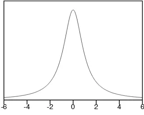
Gaussian Random Variables: A random variableX is Gaussian, also known asnormal, with parametersµ∈Randσ2 >0if its pdf is as follows
f(x) = √ 1
2πσ2exp(−
1 2(
x−µ
σ )
2
) (2.31)
whereπ = 3.1415· · ·,µis a parameter that controls the location of the center of the function andσ is a parameter than controls the spread of the function.. Here-after whenever we want to say that a random variableXis normal with parameters
µand σ2 we shall write it as X
∼ N(µ, σ2). If a Gaussian random variable X
has zero mean and standard deviation equal to one, we say that it is astandard Gaussian random variable, and represent itX∼N(0,1).
The Gaussian pdf is very important because of its ubiquitousness in nature thus the name “Normal”. The underlying reason why this distribution is so widespread in nature is explained by an important theorem known asthe central limit theo-rem. We will not prove this theorem here but it basically says that observations which are the result of a sum of a large number of random and independent in-fluences have a cumulative distribution function closely approximated by that of a Gaussian random variable. Note this theorem applies to many natural observa-tions: Height, weight, voltagefluctuations, IQ... All these variables are the result of a multitude of effects which when added up make the observations distribute approximately Gaussian.
One important property of Gaussian random variables is that linear combi-nations of Gaussian random variables produce Gaussian random variables. For example, ifX1andX2are random variables, thenY = 2 + 4X1+ 6X2would also
be a Gaussian random variable.
2.3
Cumulative Distribution Function.
The cumulative distribution function, of a random variableX is a functionFX :
R→[0,1]such that
FX(u) = P({X≤u}) (2.32)
2.3. CUMULATIVE DISTRIBUTION FUNCTION. 33
FX(u) =
0.0 ifu <0.0
1/4 ifu≥ 0.0andu <1 3/4 ifu≥ 1andu <2 1.0 ifu≥ 2
(2.33)
The relationship between the cumulative distribution function, the probability mass function and the probability density function is as follows:
FX(u) =
% .
x≤upX(u) ifX is a discrete random variable
/u
−∞fX(x)dx ifX is a continuous random variable
(2.34)
Example: To calculate the cumulative distribution function of a continuous ex-ponential random variableX with parameterλ > 0we integrate the exponential pdf
FX(u) =
%/u
0 λexp(−λx)dx ifu≥0
0 else (2.35)
And solving the integral
+ u
0
λexp(−λx)dx =
0
−exp(−λx)
1u
0
= 1−exp(−λu) (2.36)
Thus the cumulative distribution of an exponential random variable is as follows
FX(u) =
%
1−exp(−λu) ifu≥0
0 else (2.37)
Observation: We have seen that if a random variable has a probability den-sity function then the cumulative denden-sity function can be obtained by integration. Conversely we can differentiate the cumulative distribution function to obtain the probability density function
fX(u) =
dFX(u)
A Property of Cumulative distribution Functions: Here is a property of cu-mulative distribution which has important applications. Consider a random vari-able X with cumulative distribution FX now suppose we define a new random
variableY such that for each outcomeω
Y(ω) = a+bX(ω) (2.39) whereaandb"= 0are real numbers. More succinctly we say
Y =a+bX (2.40)
If we know the cumulative distribution ofY we can easily derive the cumulative distribution ofY.
FY(u) =P(Y ≤u) =P(a+bX ≤u) = P(X ≤
u−a
b }) =FX( u−a
b )
(2.41)
Example: LetXbe an exponential random variable with parameterλ, i.e.,
FX(u) =
%
0 ifu <0
1−exp(−λu) ifu≥0 (2.42)
LetY = 1 + 2X. In this casea = 1andb = 2. Thus the cumulative distribution ofY is
FY(u) =FX((u−1)/2) =
%
0 if(u−1)/2<0 1−exp(−λ(u−1)/2) if(u−1)/2≥0
(2.43)
2.4
Exercises
1. Distinguish the following standard symbolsP,pX,FX,fX,X,x
2. Find the cumulative distribution function of a Bernoulli random variableX
with parameterµ.
2.4. EXERCISES 35
4. Consider a uniform random variable in the interval[0,1]. (a) Calculate the probability of the interval[0.1,0.2]
(b) Calculate the probability of 0.5.
5. LetXbe a random variable with probability mass function
pX(u) =
%
1/5 ifu∈ {1,2,3,4,5}
0 else (2.44)
(a) FindFX(4)
(b) FindP({X ≤3} ∩ {X ≤4})
(c) Plot the functionhX(t) =P({X =t} | {X ≥t})fort = 1,2,3,4,5.
This function is commonly known as the “hazard function” ofX. If you think ofX as the life time of a system, hX(t)tells us the
proba-bility that the system fails at timet given that it has not failed up to timet. For example, the hazard function of human beings looks like a U curve with a extra bump at the teen-years and with a minimum at about 30 years.
6. LetXbe a continuous random variable with pdf
fX(u) =
0.25 ifu∈[−3,−1] 0.25 ifu∈[1,3] 0 else
(2.45)
(a) Plot fX. Can it be a probability density function? Justify your
re-sponse. (b) PlotFX
7. Show that ifXis a continuous random variable with pdffX andY =a+bX
where anda, bare real numbers. Then
fY(v) = (1/b)fX(
u−a
b ) (2.46)
hint: Work with cumulative distributions and then differentiate them to get densities.
8. Show that ifX ∼N(µ, σ2)
Chapter 3
Random Vectors
In many occasions we need to model the joint behavior of more than one variable. For example, we may want to describe whether two different stocks tend to fl uc-tuate in a somewhat linked manner or whether high levels of smoking covary with high lung cancer rates. In this chapter we examine the joint behavior of more than one random variables. To begin with, we will start working with pairs of random variables.
3.1
Joint probability mass functions
The joint probability mass function of the random variablesXandY is a function
pX,Y :R2 →[0,1], such that for all(u, v)∈R2
pX,Y(u, v) =P({X =u} ∩ {Y =v}) (3.1)
hereafter, we use the simplified notationP(X =u, Y =u)to representP({X =
u} ∩ {Y =v}), i.e., the probability measure of the set
{ω: (X(ω) = u)and(Y(ω) =v)} (3.2)
3.2
Joint probability density functions
The joint probability density function of the continuous random variablesX and
Y is a function fX,Y : R2 → [0,∞) such that for all (u, v) ∈ R2 and for all
(∆u,∆v)∈R2
P(X∈[u, u+ ∆u], Y ∈[v, v+ ∆v]) =
+ u+∆u
u
+ v+∆v
v
fX,Y(u, v)dv du (3.3)
Interpretation Note if∆uand∆vare so small thatfX,Y(u, v)is approximately
constant over the area of integration then
P(X ∈[u, u+ ∆u], Y ∈[v, v+ ∆v])≈fX,Y(u, v)∆u∆v (3.4)
In other words, the probability that (X, Y) take values in the rectangle [u, u+ ∆u]×[v, v+ ∆v]is approximately the area of the rectangle times the density at a point in the rectangle.
3.3
Joint Cumulative Distribution Functions
The joint cumulative distribution of two random variablesX andY is a function
FX,Y :R2 →[0,1]such that
FX,Y(u, v) =P({X ≤u} ∩ {Y ≤v}) (3.5)
note ifX andY are discrete then
FX,Y(u, v) =
&
x≤u
&
y≤v
pX,Y(u, v) (3.6)
and ifX andY are continuous then
FX,Y(u, v) =
+ u
−∞
+ v
−∞
fX,Y(u, v)dv du (3.7)
3.4
Marginalizing
In many occasions we know the joint probability density or probability mass func-tion of two random variablesX and Y and we want to get the probability den-sity/mass of each of the variables in isolation. Such a process is called marginal-ization and it works as follows:
pX(u) =
&
v∈R
3.5. INDEPENDENCE 39
and if the random variables are continuous
fX(u) =
+ ∞
−∞
fX,Y(u, v)dv (3.9)
Proof: Consider the functionh:R→R
h(u) =
+ ∞
−∞
fX,Y(u, v)dv (3.10)
We want to show that h is the probability density function of X. Note for all
a, b∈Rsuch thata≤b
P(X ∈[a, b]) =P(X ∈[a, b], Y ∈R) =
+ b
a
fX,Y(u, v)dv du=
+ b
a
h(u)du
(3.11) showing thathis indeed the probability density function ofX. A similar argument can be made for the discrete case.
3.5
Independence
Intuitively, two random variables X andY are independent if knowledge about one of the variables gives us no information whatsoever about the other variable. More precisely, the random variables X andY are independent if and only if all events of the form{X ∈[u, u+∆u]}and all events of the form{Y ∈[v, v+∆v]}
are independent. If the random variable is continuous, a necessary and sufficient condition for independence is that the joint probability density be the product of the densities of each variable
fX,Y(u, v) =fX(u)fY(v) (3.12)
for allu, v ∈R. If the random variable is discrete, a necessary and sufficient
con-dition for independence is that the joint probability mass function be the product of the probability mass for each of the variables
pX,Y(u, v) =pX(u)pY(v) (3.13)
3.6
Bayes’ Rule for continuous data and discrete
hy-potheses
Perhaps the most common application of Bayes’ rule occurs when the data are represented by a continuous random variableX, and the hypotheses by a discrete random variableH. In such case, Bayes’ rule works as follows
pH|X(i|u) =
fX|H(u|i)pH(i)
fX(u)
(3.14)
wherepH|X : R2 → [0,1]is known as the conditional probability mass function
ofHgivenXand it is defined as follows
pH|X(i|u) = lim
∆u→0P(H =i|X ∈[u, u+ ∆u]) (3.15)
fX|H : R2 → R+ is known as the conditional probability density function ofX givenHand it is defined as follows: For alla, b∈Rsuch thata≤b,
P(X∈[a, b]|H =i) =
+ b
a
fX|H(u|i)du (3.16)
Proof: Applying Bayes’ rule to the events{H =i}and{X ∈[u, u+ ∆u]}
P(H =i|X ∈[u, u+ ∆u]) = P(X ∈[u, u+ ∆u]|H =i)P(H =i)
P(X ∈[u, u+ ∆u]) (3.17) =
/u+∆u
u fX|H(x|i)dx P(H =i)
/u+∆u
u fX(x)dx
(3.18)
Taking limits and approximating areas with rectangles
lim
∆u→0P(H =i|X ∈[u, u+ ∆u]) =
∆ufX|H(u|i)pH(i) ∆ufX(u)
(3.19)
3.6. BAYES’ RULE FOR CONTINUOUS DATA AND DISCRETE HYPOTHESES41
3.6.1
A useful version of the LTP
In many cases we are not given fX directly and we need to compute it using
fX|H and pH. This can be done using the following version of the law of total
probability:
fX(u) =
&
j∈Range(H)
pH(j)fX|H(u|j) (3.20)
Proof: Note that for alla, b∈R, witha≤b
+ b
a
&
j∈Range(H)
pH(j)fX|H(u|j)du=
&
j∈Range(H)
pH(j)
+ b
a
fX|H(u|j)du (3.21)
= & j∈Range(H)
pH(j)P(X ∈[a, b]|H =j) =P(X ∈[a, b]) (3.22)
and thus.
j∈Range(H)pH(j)fX|H(u|j)is the probability density ofX.
Example: LetH be a Bernoulli random variable with parameterµ = 0.5. Let
Y0 ∼N(0,1),Y1 ∼N(1,1)and
X = (1−H)(Y0) + (H)(Y1) (3.23) Thus,
pH(0) =pH(1) = 0.5 (3.24)
fX|H(u|i) = 1
√
2πe
−(u−i)2
/2 fori
∈ {1,2}. (3.25) Suppose we are given the value u ∈ Rand we want to know the posterior
prob-ability thatH takes the value 0 given thatX took the valueu. To do so,first we apply LTP to computefX(u)
fX(u) = (0.5) 1
√
2π
)
e−u2/2+e−(u−1)2/2
*
= (0.5)√1
2πe
u2 /2
)
1 +e2u−1
*
(3.26) Applying Bayes’ rule,
pH|X(0|u) =
1
1 +e−(1−2u) (3.27) So, for example, ifu= 0.5the probability thatHtakes the value0is 0.5. Ifu= 1
3.7
Random Vectors and Stochastic Processes
A random vector is a collection of random variables organized as a vector. For example ifX1, . . . , Xnare random variables then
X = (X1, Y, . . . , Xn)$ (3.28)
is a random vector. A stochastic process is an ordered set of random vectors. For example, ifI is an indexing set andXt, is a random vector for allt ∈Ithen
X = (Xi :i∈ I) (3.29)
is a random process. When the indexing set is countable,Y is called a “discrete time” stochastic process. For example,
X = (X1, Y, X3, . . .) (3.30)
is a discrete time random process. If the indexing set are the real numbers, then
Y is called a “continuous time” stochastic process. For example, ifXis a random variable, the ordered set of random vectors
X= (Xt:t∈R) (3.31)
with
Chapter 4
Expected Values
The expected value (or mean) of a random variable is a generalization of the notion of arithmetic mean. It is a number that tells us about the “center of gravity” or average value we would expect to obtain is we averaged a very large number of observations from that random variable. The expected value of the random variable X is represented asE(X)or with the Greek letter µ, as in µX and it is
defined as follows
E(X) = µX =
% .
u∈RpX(u)u for discrete ravs
/+∞
−∞ pX(u)u du for continuous ravs
(4.1)
We also define the expected value of a number as the number itself, i.e., for all
u∈R
E(u) = u (4.2)
Example: The expected value of a Bernoulli random variable with parameterµ
is as follows
E(X) = (1−µ)(0.0) + (µ)(1.0) = µ (4.3)
Example: A random variableXwith the following pdf
pX(u) =
%
1
b−a ifu∈[a, b]
0 ifu"∈[a, b] (4.4)
is known as a uniform[0,1]continuous random variable. Its expected value is as follows
E(X) =
+ ∞
−∞
pX(u)u du=
+ b
a 1
b−au du
= 1
(b−a)
,u2
2
-b
a =
= 1
(b−a)(
b2−a2
2 ) = (a+b)/2 (4.5)
Example: The expected value of an exponential random variable with param-eterλis as follows (see previous chapter for definition of an exponential random variable)
E(X) =
+ ∞
−∞
upX(u)du=
+ ∞
0
uλexp(−λu)du (4.6) and using integration by parts
E(X) =,−uexp(−λu)-∞
0 +
+ ∞
0
λexp(−λu)du =−,λexp(−λu)-∞
0 =
1
λ
(4.7)
4.1
Fundamental Theorem of Expected Values
This theorem is very useful when we have a random variableY which is a function of another random variableX. In many cases we may know the probability mass function, or density function, forX but not for Y. The fundamental theorem of expected values allows us to get the expected value ofY even though we do not know the probability distribution of Y. First we’ll see a simple version of the theorem and then we will see a more general version.
Simple Version of the Fundamental Theorem: LetX : Ω→ Rbe a rav and
h:R→Ra function. LetY be a rav defined as follows:
Y(ω) =h(X(ω))for allω ∈R (4.8)
or more succinctly
4.1. FUNDAMENTAL THEOREM OF EXPECTED VALUES 45
Then it can be shown that
E(Y) =
% .
u∈RpX(u)h(u) for discrete ravs
/+∞
−∞ pX(u)h(u)du for continuous ravs
(4.10)
Example: Let X be a Bernoulli rav andY a random variable defined asY = (X−0.5)2. To
find the expected value ofY we can apply the fundamental theorem of expected values withh(u) = (u−0.5)2. Thus,
E(Y) =& u∈R
pX(u)(u−0.5)2 =pX(0)(0−0.5)2+pX(1)(1−0.5)2
= (0.5)(0.5)2+ (0.5)(−0.5)2 = 0.25 (4.11)
Example: The average entropy, or information value (in bits) of a random vari-ableXis represented asH(X)and is defined as follows
H(X) =−E(log2pX(X)) (4.12)
To find the entropy of a Bernoulli random variableX with parameter µwe can apply the fundamental theorem of expected values using the function h(u) = log2pX(u). Thus,
H(X) = & u∈R
pX(u) log2pX(u) =pX(0) log2pX(0) +pX(1) log2pX(1)
= (µ) log2(µ) + (1−µ) log2(1−µ) (4.13) For example, ifµ= 0.5, then
H(X) = (0.5) log2(0.5) + (0.5) log2(0.5) = 1bit (4.14)
General Version of the Fundamental Theorem: Let X1, . . . , Xn be random
variables, letY =h(X1, . . . , Xn), whereh:Rn→Ris a function. Then
E(Y) =
% .
(u1, . . . , un)∈RnpX1,...,Xn(u1, . . . , un)h(u1, . . . , un) for discrete ravs
/+∞
−∞ · · ·
/+∞
4.2
Properties of Expected Values
LetXandY be two random variables andaandbtwo real numbers. Then
E(X+Y) =E(X) +E(Y) (4.16) and
E(a+bX) =a+bE(X) (4.17) Moreover ifXandY are independent then
E(XY) =E(X)E(Y) (4.18) We will prove these properties using discrete ravs. The proofs are analogous for continuous ravs but substituting sums by integrals.
Proof: By the fundamental theorem of expected values
E(X+Y) =& u∈R
&
v∈R
pX,Y(u, v)(u+v)
= (& u∈R
u&
v∈R
pX,Y(u, v)) + (
&
v∈R
v&
u∈R
pX,Y(u, v))
=& u∈R
upX(u) +
&
v∈R
vpY(v) =E(X) +E(Y) (4.19)
where we used the law of total probability in the last step.
Proof: Using the fundamental theorem of expected values
E(a+bX) =& u
pX(u)(a+bu)
=a&
u∈R
pX(u) +b
&
u
upX(u) =a+bE(X) (4.20)
Proof: By the fundamental theorem of expected values
E(XY) =& u∈R
&
v∈R
pX,Y(u, v)uv (4.21)
ifXandY are independent thenpX,Y(u, v) = pX(u)pY(v). Thus
E(XY) = [& u
upX(u)] [
&
v
vpY(v)] = E(X)E(Y) (4.22)
4.3. VARIANCE 47
4.3
Variance
The variance of a random variable X is a number that represents the amount of variability in that random variable. It is defined as the expected value of the squared deviations from the mean of the random variable and it is represented as Var(X)or asσ2
X
Var(X) =σX2 =E[(X−µX)2] =
% .
u∈RpX(u)(u−µX)2 for discrete ravs
/+∞
−∞ pX(u)(u−µX)
2du for continuous ravs (4.23) Thestandard deviationof a random variableXis represented as Sd(X)orσand it is the square root of the variance of that random variable
Sd(X) =σX =
2
Var(X) (4.24)
The standard deviation is easier to interpret than the variance for it uses the same units of measurement taken by the random variable. For example if the random variable X represents reaction time in seconds, then the variance is measured in seconds squares, which is hard to interpret, while the standard deviation is measured in seconds. The standard deviation can be interpreted as a “typical” deviation from the mean. If an observation deviates from the mean by about one standard deviation, we say that that amount of deviation is “standard”.
Example: The variance of a Bernoulli random variable with parameter µis as follows
Var(X) = (1−µ)(0.0−µ)2+ (µ)(1.0−µ)2 = (µ)(1−µ) (4.25)
Example: For a continuous uniform[a, b]random variableX, the pdf is as fol-lows
pX(u) =
%
1
b−a ifu∈[a, b]
0 ifu"∈[a, b] (4.26)
which we have seen as expected valueµX = (a+b)/2. Its variance is as follows
σX2 =
+ +∞
−∞
upX(u)du= 1
b−a
+ b
a
and doing a change of varia