of Computer Programming
by
Peter Van Roy
Seif Haridi
The MIT Press
All rights reserved. No part of this book may be reproduced in any form by any electronic or mechanical means (including photocopying,recording,or information storage and retrieval) without permission in writing from the publisher.
This book was set in LATEX 2εby the authors and was printed and bound in the United States of
America.
Library of Congress Cataloging-in-Publication Data Van Roy,Peter.
Concepts,techniques,and models of computer programming / Peter Van Roy,Seif Haridi p. cm.
Includes bibliographical references and index. ISBN 0-262-22069-5
1. Computer programming. I. Haridi,Seif. II. Title.
QA76.6.V36 2004
Preface xiii
Running the Example Programs xxix
1 Introduction to Programming Concepts 1
I GENERAL COMPUTATION MODELS 27
2 Declarative Computation Model 29
3 Declarative Programming Techniques 111
4 Declarative Concurrency 233
5 Message-Passing Concurrency 345
6 Explicit State 405
7 Object-Oriented Programming 489
8 Shared-State Concurrency 569
9 Relational Programming 621
II SPECIALIZED COMPUTATION MODELS 677
10 Graphical User Interface Programming 679
11 Distributed Programming 707
12 Constraint Programming 749
III SEMANTICS 777
IV APPENDIXES 813
A Mozart System Development Environment 815
B Basic Data Types 819
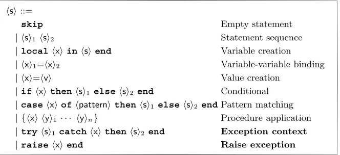
C Language Syntax 833
D General Computation Model 843
References 853
Preface xiii
Running the Example Programs xxix
1 Introduction to Programming Concepts 1
1.1 A calculator . . . 1
1.2 Variables . . . 2
1.3 Functions . . . 2
1.4 Lists . . . 4
1.5 Functions over lists . . . 7
1.6 Correctness . . . 9
1.7 Complexity . . . 10
1.8 Lazy evaluation . . . 11
1.9 Higher-order programming . . . 13
1.10 Concurrency . . . 14
1.11 Dataflow . . . 15
1.12 Explicit state . . . 16
1.13 Objects . . . 17
1.14 Classes . . . 18
1.15 Nondeterminism and time . . . 20
1.16 Atomicity . . . 21
1.17 Where do we go from here? . . . 22
1.18 Exercises . . . 23
I GENERAL COMPUTATION MODELS 27 2 Declarative Computation Model 29 2.1 Defining practical programming languages ... 30
2.2 The single-assignment store . . . 42
2.3 Kernel language . . . 49
2.4 Kernel language semantics ... 56
2.5 Memory management . . . 72
2.6 From kernel language to practical language ... 79
2.8 Advanced topics . . . 96
2.9 Exercises . . . 107
3 Declarative Programming Techniques 111 3.1 What is declarativeness? . . . 114
3.2 Iterative computation . . . 118
3.3 Recursive computation . . . 124
3.4 Programming with recursion . . . 127
3.5 Time and space efficiency . . . 166
3.6 Higher-order programming ...177
3.7 Abstract data types . . . 195
3.8 Nondeclarative needs . . . 210
3.9 Program design in the small ...218
3.10 Exercises . . . 230
4 Declarative Concurrency 233 4.1 The data-driven concurrent model . . . 235
4.2 Basic thread programming techniques ...246
4.3 Streams . . . 256
4.4 Using the declarative concurrent model directly ...272
4.5 Lazy execution . . . 278
4.6 Soft real-time programming ...304
4.7 The Haskell language . . . 308
4.8 Limitations and extensions of declarative programming ...313
4.9 Advanced topics . . . 326
4.10 Historical notes . . . 337
4.11 Exercises . . . 338
5 Message-Passing Concurrency 345 5.1 The message-passing concurrent model ...347
5.2 Port objects . . . 350
5.3 Simple message protocols ...353
5.4 Program design for concurrency ...362
5.5 Lift control system . . . 365
5.6 Using the message-passing model directly ...377
5.7 The Erlang language . . . 386
5.8 Advanced topic . . . 394
5.9 Exercises . . . 399
6 Explicit State 405 6.1 What is state? . . . 408
6.2 State and system building . . . 410
6.3 The declarative model with explicit state ...413
6.4 Data abstraction . . . 419
6.6 Reasoning with state . . . 440
6.7 Program design in the large ...450
6.8 Case studies . . . 463
6.9 Advanced topics . . . 479
6.10 Exercises . . . 482
7 Object-Oriented Programming 489 7.1 Inheritance . . . 491
7.2 Classes as complete data abstractions ...492
7.3 Classes as incremental data abstractions ...502
7.4 Programming with inheritance . . . 518
7.5 Relation to other computation models ...537
7.6 Implementing the object system . . . 545
7.7 The Java language (sequential part) . . . 551
7.8 Active objects . . . 556
7.9 Exercises . . . 567
8 Shared-State Concurrency 569 8.1 The shared-state concurrent model . . . 573
8.2 Programming with concurrency ...573
8.3 Locks . . . 582
8.4 Monitors . . . 592
8.5 Transactions . . . 600
8.6 The Java language (concurrent part) ...615
8.7 Exercises . . . 618
9 Relational Programming 621 9.1 The relational computation model ...623
9.2 Further examples . . . 627
9.3 Relation to logic programming ...631
9.4 Natural language parsing ...641
9.5 A grammar interpreter . . . 650
9.6 Databases . . . 654
9.7 The Prolog language ...660
9.8 Exercises . . . 671
II SPECIALIZED COMPUTATION MODELS 677 10 Graphical User Interface Programming 679 10.1 The declarative/procedural approach ...681
10.2 Using the declarative/procedural approach ...682
10.3 The Prototyper interactive learning tool ...689
10.4 Case studies . . . 690
10.6 Exercises . . . 703
11 Distributed Programming 707 11.1 Taxonomy of distributed systems ...710
11.2 The distribution model . . . 712
11.3 Distribution of declarative data ...714
11.4 Distribution of state . . . 720
11.5 Network awareness . . . 723
11.6 Common distributed programming patterns ...724
11.7 Distribution protocols . . . 732
11.8 Partial failure . . . 739
11.9 Security . . . 743
11.10 Building applications . . . 745
11.11 Exercises . . . 746
12 Constraint Programming 749 12.1 Propagate-and-search ...750
12.2 Programming techniques . . . 755
12.3 The constraint-based computation model ...758
12.4 Defining and using computation spaces ...762
12.5 Implementing the relational computation model ...772
12.6 Exercises . . . 774
III SEMANTICS 777 13 Language Semantics 779 13.1 The general computation model ...780
13.2 Declarative concurrency . . . 804
13.3 Eight computation models . . . 806
13.4 Semantics of common abstractions ...808
13.5 Historical notes . . . 808
13.6 Exercises . . . 809
IV APPENDIXES 813 A Mozart System Development Environment 815 A.1 Interactive interface . . . 815
A.2 Command line interface . . . 817
B Basic Data Types 819 B.1 Numbers (integers, floats, and characters) ...819
B.2 Literals (atoms and names) . . . 824
B.4 Chunks (limited records) . . . 828
B.5 Lists . . . 828
B.6 Strings . . . 830
B.7 Virtual strings . . . 831
C Language Syntax 833 C.1 Interactive statements . . . 834
C.2 Statements and expressions . . . 834
C.3 Nonterminals for statements and expressions ...836
C.4 Operators . . . 836
C.5 Keywords . . . 839
C.6 Lexical syntax . . . 839
D General Computation Model 843 D.1 Creative extension principle . . . 844
D.2 Kernel language . . . 845
D.3 Concepts . . . 846
D.4 Different forms of state . . . 849
D.5 Other concepts . . . 850
D.6 Layered language design . . . 850
References 853
Six blind sages were shown an elephant and met to discuss their experience. “It’s wonderful,” said the first, “an elephant is like a rope: slender and flexible.” “No, no, not at all,” said the second, “an elephant is like a tree: sturdily planted on the ground.” “Marvelous,” said the third, “an elephant is like a wall.” “Incredible,” said the fourth, “an elephant is a tube filled with water.” “What a strange piecemeal beast this is,” said the fifth. “Strange indeed,” said the sixth, “but there must be some underlying harmony. Let us investigate the matter further.” — Freely adapted from a traditional Indian fable.
A programming language is like a natural, human language in that it favors certain metaphors, images, and ways of thinking.
—Mindstorms: Children, Computers, and Powerful Ideas, Seymour Papert (1980)
One approach to the study of computer programming is to study programming languages.But there are a tremendously large number of languages, so large that it is impractical to study them all.How can we tackle this immensity? We could pick a small number of languages that are representative of different programming paradigms.But this gives little insight into programming as a unified discipline. This book uses another approach.
We focus on programming concepts and the techniques in using them, not on programming languages.The concepts are organized in terms of computation mod-els.A computation model is a formal system that defines how computations are done.There are many ways to define computation models.Since this book is in-tended to be practical, it is important that the computation model be directly useful to the programmer.We therefore define it in terms of concepts that are important to programmers: data types, operations, and a programming language. The termcomputation modelmakes precise the imprecise notion of “programming paradigm.” The rest of the book talks about computation models and not program-ming paradigms.Sometimes we use the phrase “programprogram-ming model.” This refers to what the programmer needs: the programming techniques and design principles made possible by the computation model.
Each computation model is based on a simple core language called its kernel lan-guage.The kernel languages are introduced in a progressive way, by adding concepts one by one.This lets us show the deep relationships between the different models. Often, adding just one new concept makes a world of difference in programming.For example, adding destructive assignment (explicit state) to functional programming allows us to do object-oriented programming.
When should we add a concept to a model and which concept should we add? We touch on these questions many times.The main criterion is thecreative extension principle.Roughly, a new concept is added when programs become complicated for technical reasons unrelated to the problem being solved.Adding a concept to the kernel language can keep programs simple, if the concept is chosen carefully.This is explained further in appendix D.This principle underlies the progression of kernel languages presented in the book.
A nice property of the kernel language approach is that it lets us use different models together in the same program.This is usually called multiparadigm pro-gramming.It is quite natural, since it means simply to use the right concepts for the problem, independent of what computation model they originate from.Mul-tiparadigm programming is an old idea.For example, the designers of Lisp and Scheme have long advocated a similar view.However, this book applies it in a much broader and deeper way than has been previously done.
From the vantage point of computation models, the book also sheds new light on important problems in informatics.We present three such areas, namely graphical user interface design, robust distributed programming, and constraint program-ming.We show how the judicious combined use of several computation models can help solve some of the problems of these areas.
Languages mentioned
We mention many programming languages in the book and relate them to particular computation models.For example, Java and Smalltalk are based on an object-oriented model.Haskell and Standard ML are based on a functional model.Prolog and Mercury are based on a logic model.Not all interesting languages can be so classified.We mention some other languages for their own merits.For example, Lisp and Scheme pioneered many of the concepts presented here.Erlang is functional, inherently concurrent, and supports fault-tolerant distributed programming.
Goals of the book
Teaching programming
The main goal of the book is to teach programming as a unified discipline with a scientific foundation that is useful to the practicing programmer.Let us look closer at what this means.
What is programming?
We defineprogramming, as a general human activity, to mean the act of extending or changing a system’s functionality.Programming is a widespread activity that is done both by nonspecialists (e.g., consumers who change the settings of their alarm clock or cellular phone) and specialists (computer programmers, the audience for this book).
This book focuses on the construction of software systems.In that setting, pro-gramming is the step between the system’s specification and a running program that implements it.The step consists in designing the program’s architecture and abstractions and coding them into a programming language.This is a broad view, perhaps broader than the usual connotation attached to the word “programming.” It covers both programming “in the small” and “in the large.” It covers both (language-independent) architectural issues and (language-dependent) coding is-sues.It is based more on concepts and their use rather than on any one program-ming language.We find that this general view is natural for teaching programprogram-ming. It is unbiased by limitations of any particular language or design methodology. When used in a specific situation, the general view is adapted to the tools used, taking into account their abilities and limitations.
Both science and technology
Programming as defined above has two essential parts: a technology and its scientific foundation.The technology consists of tools, practical techniques, and standards, allowing us to do programming.The science consists of a broad and deep theory with predictive power, allowing us to understand programming.Ideally, the science should explain the technology in a way that is as direct and useful as possible.
More than a craft
Despite many efforts to introduce a scientific foundation, programming is almost always taught as a craft.It is usually taught in the context of one (or a few) programming language(s) (e.g., Java, complemented with Haskell, Scheme, or Pro-log).The historical accidents of the particular languages chosen are interwoven to-gether so closely with the fundamental concepts that the two cannot be separated. There is a confusion between tools and concepts.What’s more, different schools of thought have developed, based on different ways of viewing programming, called “paradigms”: object-oriented, logic, functional, etc.Each school of thought has its own science.The unity of programming as a single discipline has been lost.
Teaching programming in this fashion is like having separate schools of bridge building: one school teaches how to build wooden bridges and another school teaches how to build iron bridges.Graduates of either school would implicitly consider the restriction to wood or iron as fundamental and would not think of using wood and iron together.
The result is that programs suffer from poor design.We give an example based on Java, but the problem exists in all languages to some degree.Concurrency in Java is complex to use and expensive in computational resources.Because of these difficulties, Java-taught programmers conclude that concurrency is a fundamentally complex and expensive concept.Program specifications are designed around the difficulties, often in a contorted way.But these difficulties are not fundamental at all.There are forms of concurrency that are quite useful and yet as easy to program with as sequential programs (e.g., stream programming as exemplified by Unix pipes).Furthermore, it is possible to implement threads, the basic unit of concurrency, almost as cheaply as procedure calls.If the programmer were taught about concurrency in the correct way, then he or she would be able to specify for and program in systems without concurrency restrictions (including improved versions of Java).
The kernel language approach
Practical programming languages scale up to programs of millions of lines of code. They provide a rich set of abstractions and syntax.How can we separate the languages’ fundamental concepts, which underlie their success, from their historical accidents? The kernel language approach shows one way.In this approach, a practical language is translated into a kernel language that consists of a small number of programmer-significant elements.The rich set of abstractions and syntax is encoded in the kernel language.This gives both programmer and student a clear insight into what the language does.The kernel language has a simple formal semantics that allows reasoning about program correctness and complexity. This gives a solid foundation to the programmer’s intuition and the programming techniques built on top of it.
small set of closely related kernel languages.It follows that the kernel language approach is a truly language-independent way to study programming.Since any given language translates into a kernel language that is a subset of a larger, more complete kernel language, the underlying unity of programming is regained.
Reducing a complex phenomenon to its primitive elements is characteristic of the scientific method.It is a successful approach that is used in all the exact sciences. It gives a deep understanding that has predictive power.For example, structural science lets one design all bridges (whether made of wood, iron, both, or anything else) and predict their behavior in terms of simple concepts such as force, energy, stress, and strain, and the laws they obey [70].
Comparison with other approaches
Let us compare the kernel language approach with three other ways to give programming a broad scientific basis:
A foundational calculus, like theλcalculus orπcalculus, reduces programming to a minimal number of elements.The elements are chosen to simplify mathematical analysis, not to aid programmer intuition.This helps theoreticians, but is not particularly useful to practicing programmers.Foundational calculi are useful for studying the fundamental properties and limits of programming a computer, not for writing or reasoning about general applications.
A virtual machine defines a language in terms of an implementation on an ideal-ized machine.A virtual machine gives a kind of operational semantics, with concepts that are close to hardware.This is useful for designing computers, implementing languages, or doing simulations.It is not useful for reasoning about programs and their abstractions.
A multiparadigm language is a language that encompasses several programming paradigms.For example, Scheme is both functional and imperative [43], and Leda has elements that are functional, object-oriented, and logical [31].The usefulness of a multiparadigm language depends on how well the different paradigms are integrated.
The kernel language approach combines features of all these approaches.A well-designed kernel language covers a wide range of concepts, like a well-well-designed multiparadigm language.If the concepts are independent, then the kernel language can be given a simple formal semantics, like a foundational calculus.Finally, the formal semantics can be a virtual machine at a high level of abstraction.This makes it easy for programmers to reason about programs.
Designing abstractions
programs but rather designing abstractions.Programming a computer is primarily designing and using abstractions to achieve new goals.We define an abstraction loosely as a tool or device that solves a particular problem.Usually the same abstraction can be used to solve many different problems.This versatility is one of the key properties of abstractions.
Abstractions are so deeply part of our daily life that we often forget about them.Some typical abstractions are books, chairs, screwdrivers, and automobiles.1 Abstractions can be classified into a hierarchy depending on how specialized they are (e.g., “pencil” is more specialized than “writing instrument,” but both are abstractions).
Abstractions are particularly numerous inside computer systems.Modern com-puters are highly complex systems consisting of hardware, operating system, mid-dleware, and application layers, each of which is based on the work of thousands of people over several decades.They contain an enormous number of abstractions, working together in a highly organized manner.
Designing abstractions is not always easy.It can be a long and painful process, as different approaches are tried, discarded, and improved.But the rewards are very great.It is not too much of an exaggeration to say that civilization is built on successful abstractions [153].New ones are being designed every day.Some ancient ones, like the wheel and the arch, are still with us.Some modern ones, like the cellular phone, quickly become part of our daily life.
We use the following approach to achieve the second goal.We start with program-ming concepts, which are the raw materials for building abstractions.We introduce most of the relevant concepts known today, in particular lexical scoping, higher-order programming, compositionality, encapsulation, concurrency, exceptions, lazy execution, security, explicit state, inheritance, and nondeterministic choice.For each concept, we give techniques for building abstractions with it.We give many exam-ples of sequential, concurrent, and distributed abstractions.We give some general laws for building abstractions.Many of these general laws have counterparts in other applied sciences, so that books like [63], [70], and [80] can be an inspiration to programmers.
Main features
Pedagogical approach
There are two complementary approaches to teaching programming as a rigorous discipline:
The computation-based approach presents programming as a way to define
executions on machines.It grounds the student’s intuition in the real world by means of actual executions on real systems.This is especially effective with an interactive system: the student can create program fragments and immediately see what they do.Reducing the time between thinking “what if” and seeing the result is an enormous aid to understanding.Precision is not sacrificed, since the formal semantics of a program can be given in terms of an abstract machine.
The logic-based approach presents programming as a branch of mathematical logic.Logic does not speak of execution but of program properties, which is a higher level of abstraction.Programs are mathematical constructions that obey logical laws.The formal semantics of a program is given in terms of a mathematical logic.Reasoning is done with logical assertions.The logic-based approach is harder for students to grasp yet it is essential for defining precise specifications of what programs do.
Like Structure and Interpretation of Computer Programs [1, 2], our book mostly uses the computation-based approach.Concepts are illustrated with program frag-ments that can be run interactively on an accompanying software package, the Mozart Programming System [148].Programs are constructed with a building-block approach, using lower-level abstractions to build higher-level ones.A small amount of logical reasoning is introduced in later chapters, e.g., for defining specifications and for using invariants to reason about programs with state.
Formalism used
This book uses a single formalism for presenting all computation models and programs, namely the Oz language and its computation model.To be precise, the computation models of the book are all carefully chosen subsets of Oz.Why did we choose Oz? The main reason is that it supports the kernel language approach well. Another reason is the existence of the Mozart Programming System.
Panorama of computation models
More is not better (or worse), just different
All computation models have their place.It is not true that models with more concepts are better or worse.This is because a new concept is like a two-edged sword.Adding a concept to a computation model introduces new forms of expres-sion, making some programs simpler, but it also makes reasoning about programs harder.For example, by adding explicit state (mutable variables) to a functional programming model we can express the full range of object-oriented programming techniques.However, reasoning about object-oriented programs is harder than rea-soning about functional programs.Functional programming is about calculating values with mathematical functions.Neither the values nor the functions change over time.Explicit state is one way to model things that change over time: it pro-vides a container whose content can be updated.The very power of this concept makes it harder to reason about.
The importance of using models together
Each computation model was originally designed to be used in isolation.It might therefore seem like an aberration to use several of them together in the same program.We find that this is not at all the case.This is because models are not just monolithic blocks with nothing in common.On the contrary, they have much in common.For example, the differences between declarative and imperative models (and between concurrent and sequential models) are very small compared to what they have in common.Because of this, it is easy to use several models together.
But even though it is technically possible, why would one want to use several models in the same program? The deep answer to this question is simple: because one does not program with models, but with programming concepts and ways to combine them.Depending on which concepts one uses, it is possible to consider that one is programming in a particular model.The model appears as a kind of epiphenomenon.Certain things become easy, other things become harder, and reasoning about the program is done in a particular way.It is quite natural for a well-written program to use different models.At this early point this answer may seem cryptic.It will become clear later in the book.
The limits of single models
We find that a good programming style requires using programming concepts that are usually associated with different computation models.Languages that implement just one computation model make this difficult:
Object-oriented languages encourage the overuse of state and inheritance.Ob-jects are stateful by default.While this seems simple and intuitive, it actually complicates programming, e.g., it makes concurrency difficult (see section 8.2). Design patterns, which define a common terminology for describing good program-ming techniques, are usually explained in terms of inheritance [66].In many cases, simpler higher-order programming techniques would suffice (see section 7.4.7). In addition, inheritance is often misused.For example, object-oriented graphical user interfaces often recommend using inheritance to extend generic widget classes with application-specific functionality (e.g., in the Swing components for Java). This is counter to separation of concerns.
Functional languages encourage the overuse of higher-order programming.Typical examples are monads and currying.Monads are used to encode state by threading it throughout the program.This makes programs more intricate but does not achieve the modularity properties of true explicit state (see section 4.8). Currying lets you apply a function partially by giving only some of its arguments.This returns a new function that expects the remaining arguments.The function body will not execute until all arguments are there.The flip side is that it is not clear by inspection whether a function has all its arguments or is still curried (“waiting” for the rest). Logic languages in the Prolog tradition encourage the overuse of Horn clause syntax and search.These languages define all programs as collections of Horn clauses, which resemble simple logical axioms in an “if-then” style.Many algorithms are obfuscated when written in this style.Backtracking-based search must always be used even though it is almost never needed (see [217]).
These examples are to some extent subjective; it is difficult to be completely objective regarding good programming style and language expressiveness.Therefore they should not be read as passing any judgment on these models.Rather, they are hints that none of these models is a panacea when used alone.Each model is well-adapted to some problems but less to others.This book tries to present a balanced approach, sometimes using a single model in isolation but not shying away from using several models together when it is appropriate.
Teaching from the book
systems.Informatics is sometimes calledcomputing.
Role in informatics curriculum
Let us consider the discipline of programming independent of any other domain in informatics.In our experience, it divides naturally into three core topics:
1.Concepts and techniques 2.Algorithms and data structures
3.Program design and software engineering
The book gives a thorough treatment of topic (1) and an introduction to (2) and (3).In which order should the topics be given? There is a strong interdependency between (1) and (3).Experience shows that program design should be taught early on, so that students avoid bad habits.However, this is only part of the story since students need to know about concepts to express their designs.Parnas has used an approach that starts with topic (3) and uses an imperative computation model [161]. Because this book uses many computation models, we recommend using it to teach (1) and (3) concurrently, introducing new concepts and design principles together. In the informatics program at the Universit´e catholique de Louvain at Louvain-la-Neuve, Belgium (UCL), we attribute eight semester-hours to each topic.This includes lectures and lab sessions.Together the three topics make up one sixth of the full informatics curriculum for licentiate and engineering degrees.
There is another point we would like to make, which concerns how to teach concurrent programming.In a traditional informatics curriculum, concurrency is taught by extending a stateful model, just as chapter 8 extends chapter 6.This is rightly considered to be complex and difficult to program with.There are other, simpler forms of concurrent programming.The declarative concurrency of chapter 4 is much simpler to program with and can often be used in place of stateful concurrency (see the epigraph that starts chapter 4).Stream concurrency, a simple form of declarative concurrency, has been taught in first-year courses at MIT and other institutions.Another simple form of concurrency, message passing between threads, is explained in chapter 5.We suggest that both declarative concurrency and message-passing concurrency be part of the standard curriculum and be taught before stateful concurrency.
Courses
We have used the book as a textbook for several courses ranging from second-year undergraduate to graduate courses [175, 220, 221].In its present form, the book is not intended as a first programming course, but the approach could likely be adapted for such a course.2 Students should have some basic programming
experience (e.g., a practical introduction to programming and knowledge of simple data structures such as sequences, sets, and stacks) and some basic mathematical knowledge (e.g., a first course on analysis, discrete mathematics, or algebra). The book has enough material for at least four semester-hours worth of lectures and as many lab sessions.Some of the possible courses are:
An undergraduate course on programming concepts and techniques.Chapter 1 gives a light introduction.The course continues with chapters 2 through 8.Depend-ing on the desired depth of coverage, more or less emphasis can be put on algorithms (to teach algorithms along with programming), concurrency (which can be left out completely, if so desired), or formal semantics (to make intuitions precise).
An undergraduate course on applied programming models.This includes rela-tional programming (chapter 9), specific programming languages (especially Erlang, Haskell, Java, and Prolog), graphical user interface programming (chapter 10), dis-tributed programming (chapter 11), and constraint programming (chapter 12).This course is a natural sequel to the previous one.
An undergraduate course on concurrent and distributed programming (chap-ters 4, 5, 8, and 11).Students should have some programming experience.The course can start with small parts of chapters 2, 3, 6, and 7 to introduce declarative and stateful programming.
A graduate course on computation models (the whole book, including the seman-tics in chapter 13).The course can concentrate on the relationships between the models and on their semantics.
The book’s Web site has more information on courses, including transparencies and lab assignments for some of them.The Web site has an animated interpreter that shows how the kernel languages execute according to the abstract machine semantics.The book can be used as a complement to other courses:
Part of an undergraduate course on constraint programming (chapters 4, 9, and 12).
Part of a graduate course on intelligent collaborative applications (parts of the whole book, with emphasis on part II).If desired, the book can be complemented by texts on artificial intelligence (e.g., [179]) or multi-agent systems (e.g., [226]).
Part of an undergraduate course on semantics.All the models are formally defined in the chapters that introduce them, and this semantics is sharpened in chapter 13. This gives a real-sized case study of how to define the semantics of a complete modern programming language.
Each chapter ends with a set of exercises that usually involve some programming. They can be solved on the Mozart system.To best learn the material in the chapter, we encourage students to do as many exercises as possible.Exercises marked (advanced exercise) can take from several days up to several weeks.Exercises marked (research project) are open-ended and can result in significant research contributions.
Software
A useful feature of the book is that all program fragments can be run on a software platform, the Mozart Programming System.Mozart is a full-featured production-quality programming system that comes with an interactive incremental devel-opment environment and a full set of tools.It compiles to an efficient platform-independent bytecode that runs on many varieties of Unix and Windows, and on Mac OS X.Distributed programs can be spread out over all these systems.The Mozart Web site, http://www.mozart-oz.org, has complete information, includ-ing downloadable binaries, documentation, scientific publications, source code, and mailing lists.
The Mozart system implements efficiently all the computation models covered in the book.This makes it ideal for using models together in the same program and for comparing models by writing programs to solve a problem in different models.Because each model is implemented efficiently, whole programs can be written in just one model.Other models can be brought in later, if needed, in a pedagogically justified way.For example, programs can be completely written in an object-oriented style, complemented by small declarative components where they are most useful.
The Mozart system is the result of a long-term development effort by the Mozart Consortium, an informal research and development collaboration of three laboratories.It has been under continuing development since 1991.The system is released with full source code under an Open Source license agreement.The first public release was in 1995.The first public release with distribution support was in 1999.The book is based on an ideal implementation that is close to Mozart version 1.3.0, released in 2003. The differences between the ideal implementation and Mozart are listed on the book’s Web site.
History and acknowledgments
Our main research vehicle and “test bed” of new ideas is the Mozart system, which implements the Oz language.The system’s main designers and developers are (in alphabetical order) Per Brand, Thorsten Brunklaus, Denys Duchier, Kevin Glynn, Donatien Grolaux, Seif Haridi, Dragan Havelka, Martin Henz, Erik Klintskog, Leif Kornstaedt, Michael Mehl, Martin M¨uller, Tobias M¨uller, Anna Neiderud, Konstantin Popov, Ralf Scheidhauer, Christian Schulte, Gert Smolka, Peter Van Roy, and J¨org W¨urtz.Other important contributors are (in alphabetical order) Ili`es Alouini, Rapha¨el Collet, Frej Drejhammer, Sameh El-Ansary, Nils Franz´en, Martin Homik, Simon Lindblom, Benjamin Lorenz, Valentin Mesaros, and Andreas Simon.We thank Konstantin Popov and Kevin Glynn for managing the release of Mozart version 1.3.0, which is designed to accompany the book.
We would also like to thank the following researchers and indirect contribu-tors: Hassan A¨ıt-Kaci, Joe Armstrong, Joachim Durchholz, Andreas Franke, Claire Gardent, Fredrik Holmgren, Sverker Janson, Torbj¨orn Lager, Elie Milgrom, Jo-han Montelius, Al-Metwally Mostafa, Joachim Niehren, Luc Onana, Marc-Antoine Parent, Dave Parnas, Mathias Picker, Andreas Podelski, Christophe Ponsard, Mah-moud Rafea, Juris Reinfelds, Thomas Sj¨oland, Fred Spiessens, Joe Turner, and Jean Vanderdonckt.
We give special thanks to the following people for their help with material related to the book.Rapha¨el Collet for co-authoring chapters 12 and 13, for his work on the practical part of LINF1251, a course taught at UCL, and for his help with the LATEX 2ε formatting.Donatien Grolaux for three graphical user interface case studies (used in sections 10.4.2–10.4.4). Kevin Glynn for writing the Haskell introduction (section 4.7). William Cook for his comments on data abstraction.Frej Drejhammar, Sameh El-Ansary, and Dragan Havelka for their help with the practical part of DatalogiII, a course taught at KTH (the Royal Institute of Technology, Stockholm).Christian Schulte for completely rethinking and redeveloping a subsequent edition of DatalogiII and for his comments on a draft of the book.Ali Ghodsi, Johan Montelius, and the other three assistants for their help with the practical part of this edition.Luis Quesada and Kevin Glynn for their work on the practical part of INGI2131, a course taught at UCL. Bruno Carton, Rapha¨el Collet, Kevin Glynn, Donatien Grolaux, Stefano Gualandi, Valentin Mesaros, Al-Metwally Mostafa, Luis Quesada, and Fred Spiessens for their efforts in proofreading and testing the example programs.We thank other people too numerous to mention for their comments on the book.Finally, we thank the members of the Department of Computing Science and Engineering at UCL, SICS (the Swedish Institute of Computer Science, Stockholm), and the Department of Microelectronics and Information Technology at KTH.We apologize to anyone we may have inadvertently omitted.
polish.3Around 1990, some of us came together with already strong system-building and theoretical backgrounds.These people initiated the ACCLAIM project, funded by the European Union (1991–1994).For some reason, this project became a focal point.Three important milestones among many were the papers by Sverker Janson and Seif Haridi in 1991 [105] (multiple paradigms in the Andorra Kernel Language AKL), by Gert Smolka in 1995 [199] (building abstractions in Oz), and by Seif Haridi et al.in 1998 [83] (dependable open distribution in Oz).The first paper on Oz was published in 1993 and already had many important ideas [89].After ACCLAIM, two laboratories continued working together on the Oz ideas: the Programming Systems Lab (DFKI, Saarland University, and Collaborative Research Center SFB 378) at Saarbr¨ucken, Germany, and the Intelligent Systems Laboratory at SICS.
The Oz language was originally designed by Gert Smolka and his students in the Programming Systems Lab [85, 89, 90, 190, 192, 198, 199].The well-factorized design of the language and the high quality of its implementation are due in large part to Smolka’s inspired leadership and his lab’s system-building expertise. Among the developers, we mention Christian Schulte for his role in coordinating general development, Denys Duchier for his active support of users, and Per Brand for his role in coordinating development of the distributed implementation.In 1996, the German and Swedish labs were joined by the Department of Computing Science and Engineering at UCL when the first author moved there.Together the three laboratories formed the Mozart Consortium with its neutral Web site http://www.mozart-oz.orgso that the work would not be tied down to a single institution.
This book was written using LATEX 2ε, flex, xfig, xv, vi/vim, emacs, and Mozart, first on a Dell Latitude with Red Hat Linux and KDE, and then on an Apple Macintosh PowerBook G4 with Mac OS X and X11.The screenshots were taken on a Sun workstation running Solaris.The first author thanks the Walloon Region of Belgium for their generous support of the Oz/Mozart work at UCL in the PIRATES and MILOS projects.
Final comments
We have tried to make this book useful both as a textbook and as a reference.It is up to you to judge how well it succeeds in this.Because of its size, it is likely that some errors remain.If you find any, we would appreciate hearing from you.Please send them and all other constructive comments you may have to the following address:
Concepts, Techniques, and Models of Computer Programming Department of Computing Science and Engineering
Universit´e catholique de Louvain B-1348 Louvain-la-Neuve, Belgium
As a final word, we would like to thank our families and friends for their support and encouragement during the four years it took us to write this book.Seif Haridi would like to give a special thanks to his parents Ali and Amina and to his family Eeva, Rebecca, and Alexander.Peter Van Roy would like to give a special thanks to his parents Frans and Hendrika and to his family Marie-Th´er`ese, Johan, and Lucile.
Louvain-la-Neuve, Belgium Peter Van Roy
Kista, Sweden Seif Haridi
This book gives many example programs and program fragments, All of these can be run on the Mozart Programming System.To make this as easy as possible, please keep the following points in mind:
The Mozart system can be downloaded without charge from the Mozart Con-sortium Web sitehttp://www.mozart-oz.org.Releases exist for various flavors of Windows and Unix and for Mac OS X.
All examples, except those intended for standalone applications, can be run in Mozart’s interactive development environment.Appendix A gives an introduction to this environment.
New variables in the interactive examples must be declared with the declare statement.The examples of chapter 1 show how to do this.Forgetting these declarations can result in strange errors if older versions of the variables exist. Starting with chapter 2 and for all following chapters, thedeclare statement is omitted in the text when it is obvious what the new variables are.It should be added to run the examples.
Some chapters use operations that are not part of the standard Mozart release. The source code for these additional operations (along with much other useful material) is given on the book’s Web site.We recommend putting these definitions in your.ozrcfile, so they will be loaded automatically when the system starts up. The book occasionally gives screenshots and timing measurements of programs. The screenshots were taken on a Sun workstation running Solaris and the timing measurements were done on Mozart 1.1.0 under Red Hat Linux release 6.1 on a Dell Latitude CPx notebook computer with Pentium III processor at 500 MHz, unless otherwise indicated.Screenshot appearance and timing numbers may vary on your system.
There is no royal road to geometry.
— Euclid’s reply to Ptolemy, Euclid (fl. c.300 B.C.) Just follow the yellow brick road.
—The Wonderful Wizard of Oz, L. Frank Baum (1856–1919)
Programming is telling a computer how it should do its job.This chapter gives a gentle, hands-on introduction to many of the most important concepts in program-ming.We assume you have had some previous exposure to computers.We use the interactive interface of Mozart to introduce programming concepts in a progressive way.We encourage you to try the examples in this chapter on a running Mozart system.
This introduction only scratches the surface of the programming concepts we will see in this book.Later chapters give a deep understanding of these concepts and add many other concepts and techniques.
1.1
A calculator
Let us start by using the system to do calculations.Start the Mozart system by typing:
oz
or by double-clicking a Mozart icon.This opens an editor window with two frames. In the top frame, type the following line:
{Browse 9999*9999}
1.2
Variables
While working with the calculator, we would like to remember an old result, so that we can use it later without retyping it.We can do this by declaring a variable:
declare V=9999*9999
This declaresVand binds it to99980001.We can use this variable later on: {Browse V*V}
This displays the answer 9996000599960001.Variables are just shortcuts for values.They cannot be assigned more than once.But you can declare another variable with the same name as a previous one.The previous variable then becomes inaccessible.Previous calculations that used it are not changed.This is because there are two concepts hiding behind the word “variable”:
The identifier.This is what you type in.Variables start with a capital letter and can be followed by any number of letters or digits.For example, the character sequenceVar1can be a variable identifier.
The store variable.This is what the system uses to calculate with.It is part of the system’s memory, which we call its store.
The declare statement creates a new store variable and makes the variable identifier refer to it.Previous calculations using the same identifier are not changed because the identifier refers to another store variable.
1.3
Functions
Let us do a more involved calculation.Assume we want to calculate the factorial functionn!, which is defined as 1×2× · · · ×(n−1)×n.This gives the number of permutations ofnitems, i.e., the number of different ways these items can be put in a row.Factorial of 10 is:
{Browse 1*2*3*4*5*6*7*8*9*10}
This displays3628800.What if we want to calculate the factorial of 100? We would like the system to do the tedious work of typing in all the integers from 1 to 100. We will do more: we will tell the system how to calculate the factorial of anyn.We do this by defining a function:
declare fun {Fact N}
if N==0 then 1 else N*{Fact N-1} end end
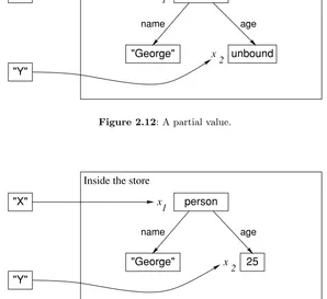
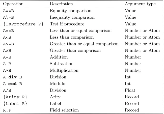
argument N, which is a local variable, i.e., it is known only inside the function body.Each time we call the function a new local variable is created.
Recursion
The function body is an instruction called anifexpression.When the function is called, then theifexpression does the following steps:
It first checks whetherNis equal to 0 by doing the testN==0.
If the test succeeds, then the expression after the then is calculated.This just returns the number 1.This is because the factorial of 0 is 1.
If the test fails, then the expression after the else is calculated.That is, ifNis not 0, then the expressionN*{Fact N-1}is calculated.This expression usesFact, the very function we are defining! This is called recursion.It is perfectly normal and no cause for alarm.
Factuses the following mathematical definition of factorial: 0! = 1
n! =n×(n−1)! if n >0
This definition is recursive because the factorial ofNisNtimes the factorial ofN-1. Let us try out the functionFact:
{Browse {Fact 10}}
This should display3628800as before.This gives us confidence thatFactis doing the right calculation.Let us try a bigger input:
{Browse {Fact 100}}
This will display a huge number (which we show in groups of five digits to improve readability):
933 26215 44394 41526 81699 23885 62667 00490 71596 82643 81621 46859 29638 95217 59999 32299 15608 94146 39761 56518 28625 36979 20827 22375 82511 85210 91686 40000 00000 00000 00000 00000
Combinations
Let us write a function to calculate the number of combinations of k items taken fromn.This is equal to the number of subsets of sizekthat can be made from a set of size n.This is writtennkin mathematical notation and pronounced “nchoose k.” It can be defined as follows using the factorial:
n k
= n!
k! (n−k)!
which leads naturally to the following function: declare
fun {Comb N K}
{Fact N} div ({Fact K}*{Fact N-K}) end
For example,{Comb 10 3}is 120, which is the number of ways that 3 items can be taken from 10.This is not the most efficient way to writeComb, but it is probably the simplest.
Functional abstraction
The definition ofCombuses the existing functionFactin its definition.It is always possible to use existing functions when defining new functions.Using functions to build abstractions is called functional abstraction.In this way, programs are like onions, with layers upon layers of functions calling functions.This style of programming is covered in chapter 3.
1.4
Lists
Now we can calculate functions of integers.But an integer is really not very much to look at.Say we want to calculate with lots of integers.For example, we would like to calculate Pascal’s triangle1:
1
1 1
1 2 1
1 3 3 1
1 4 6 4 1
. . . .
1. Pascal’s triangle is a key concept in combinatorics. The elements of the nth row are the combinations`n
k
´
, wherekranges from 0 ton. This is closely related to the binomial theorem, which states (x+y)n=Pn
k=0 `n
k
´
nil
2
1 2
1 2
1 2
1 2
1 2
1 2
8 nil
1
5 |
L = [5 6 7 8]
L =
L.2 =
L.1 = 5
L.2 = [6 7 8]
|
6 |
7 |
8
|
6 |
7 |
Figure 1.1: Taking apart the list[5 6 7 8].
This triangle is named after scientist and philosopher Blaise Pascal.It starts with 1 in the first row.Each element is the sum of the two elements just above it to the left and right.(If there is no element, as on the edges, then zero is taken.) We would like to define one function that calculates the whole nth row in one swoop. The nth row hasnintegers in it.We can do it by using lists of integers.
A list is just a sequence of elements, bracketed at the left and right, like[5 6 7 8].For historical reasons, the empty list is writtennil(and not []).Lists can be displayed just like numbers:
{Browse [5 6 7 8]}
The notation[5 6 7 8]is a shortcut.A list is actually a chain of links, where each link contains two things: one list element and a reference to the rest of the chain. Lists are always created one element at a time, starting withniland adding links one by one. A new link is written H|T, where H is the new element and T is the old part of the chain.Let us build a list.We start withZ=nil.We add a first link Y=7|Zand then a second linkX=6|Y.Now Xreferences a list with two links, a list that can also be written as[6 7].
The linkH|T is often called a cons, a term that comes from Lisp.2 We also call it a list pair.Creating a new link is called consing.IfTis a list, then consingHand Ttogether makes a new list H|T:
1
2
1
Third row1
1
Second row1
First row(0)
1
3
3
1
(0)
1
4
6
4
1
+
+
+
+
+
Fourth row
Fifth row
Figure 1.2: Calculating the fifth row of Pascal’s triangle.
declare H=5 T=[6 7 8] {Browse H|T}
The listH|Tcan be written[5 6 7 8].It has head 5and tail[6 7 8].The cons H|Tcan be taken apart, to get back the head and tail:
declare L=[5 6 7 8] {Browse L.1} {Browse L.2}
This uses the dot operator “.”, which is used to select the first or second argument of a list pair.DoingL.1gives the head ofL, the integer5.DoingL.2gives the tail of L, the list [6 7 8].Figure 1.1 gives a picture: L is a chain in which each link has one list element andnil marks the end.DoingL.1gets the first element and doingL.2gets the rest of the chain.
Pattern matching
A more compact way to take apart a list is by using the case instruction, which gets both head and tail in one step:
declare L=[5 6 7 8]
case L of H|T then {Browse H} {Browse T} end
1.5
Functions over lists
Now that we can calculate with lists, let us define a function, {Pascal N}, to calculate the nth row of Pascal’s triangle.Let us first understand how to do the calculation by hand.Figure 1.2 shows how to calculate the fifth row from the fourth. Let us see how this works if each row is a list of integers.To calculate a row, we start from the previous row.We shift it left by one position and shift it right by one position.We then add the two shifted rows together.For example, take the fourth row:
[1 3 3 1]
We shift this row left and right and then add them together element by element:
[1 3 3 1 0 ] + [0 1 3 3 1]
Note that shifting left adds a zero to the right and shifting right adds a zero to the left.Doing the addition gives
[1 4 6 4 1]
which is the fifth row.
The main function
Now that we understand how to solve the problem, we can write a function to do the same operations.Here it is:
declare Pascal AddList ShiftLeft ShiftRight fun {Pascal N}
if N==1 then [1] else
{AddList {ShiftLeft {Pascal N-1}} {ShiftRight {Pascal N-1}}} end
end
In addition to defining Pascal, we declare the variables for the three auxiliary functions that remain to be defined.
The auxiliary functions
fun {ShiftLeft L} case L of H|T then
H|{ShiftLeft T} else [0] end end
fun {ShiftRight L} 0|L end
ShiftRightjust adds a zero to the left. ShiftLefttraversesL one element at a time and builds the output one element at a time.We have added anelse to the caseinstruction.This is similar to an elsein anif: it is executed if the pattern of thecasedoes not match.That is, whenLis empty, then the output is[0], i. e. , a list with just zero inside.
Here isAddList: fun {AddList L1 L2}
case L1 of H1|T1 then case L2 of H2|T2 then
H1+H2|{AddList T1 T2} end
else nil end end
This is the most complicated function we have seen so far.It uses two case instructions, one inside another, because we have to take apart two lists, L1 and L2.Now we have the complete definition of Pascal.We can calculate any row of Pascal’s triangle.For example, calling{Pascal 20}returns the 20th row:
[1 19 171 969 3876 11628 27132 50388 75582 92378 92378 75582 50388 27132 11628 3876 969 171 19 1]
Is this answer correct? How can we tell? It looks right: it is symmetric (reversing the list gives the same list) and the first and second arguments are 1 and 19, which are right.Looking at figure 1.2, it is easy to see that the second element of the nth row is alwaysn−1 (it is always one more than the previous row and it starts out zero for the first row).In the next section, we will see how to reason about correctness.
Top-down software development
Let us summarize the methodology we used to writePascal: The first step is to understand how to do the calculation by hand.
The second step is to write a main function to solve the problem, assuming that some auxiliary functions are known (here,ShiftLeft,ShiftRight, andAddList).
The third step is to complete the solution by writing the auxiliary functions.
1.6
Correctness
A program is correct if it does what we would like it to do.How can we tell whether a program is correct? Usually it is impossible to duplicate the program’s calculation by hand.We need other ways.One simple way, which we used before, is to verify that the program is correct for outputs that we know.This increases confidence in the program.But it does not go very far.To prove correctness in general, we have to reason about the program.This means three things:
We need a mathematical model of the operations of the programming language, defining what they should do.This model is called the language’s semantics.
We need to define what we would like the program to do.Usually, this is a mathematical definition of the inputs that the program needs and the output that it calculates.This is called the program’s specification.
We use mathematical techniques to reason about the program, using the seman-tics.We would like to demonstrate that the program satisfies the specification.
A program that is proved correct can still give incorrect results, if the system on which it runs is incorrectly implemented.How can we be confident that the system satisfies the semantics? Verifying this is a major undertaking: it means verifying the compiler, the run-time system, the operating system, the hardware, and the physics upon which the hardware is based! These are all important tasks, but they are beyond the scope of the book.We place our trust in the Mozart developers, software companies, hardware manufacturers, and physicists.3
Mathematical induction
One very useful technique is mathematical induction.This proceeds in two steps. We first show that the program is correct for the simplest case.Then we show that, if the program is correct for a given case, then it is correct for the next case.If we can be sure that all cases are eventually covered, then mathematical induction lets us conclude that the program is always correct.This technique can be applied for integers and lists:
For integers, the simplest case is 0 and for a given integernthe next case isn+ 1. For lists, the simplest case isnil(the empty list) and for a given listTthe next case isH|T(with no conditions onH).
Let us see how induction works for the factorial function:
{Fact 0}returns the correct answer, namely 1.
Assume that{Fact N-1}is correct.Then look at the call{Fact N}.We see that theifinstruction takes theelsecase (sinceNis not zero), and calculatesN*{Fact N-1}.By hypothesis, {Fact N-1} returns the right answer.Therefore, assuming that the multiplication is correct,{Fact N}also returns the right answer.
This reasoning uses the mathematical definition of factorial, namelyn! =n×(n−1)! if n > 0, and 0! = 1.Later in the book we will see more sophisticated reasoning techniques.But the basic approach is always the same: start with the language semantics and problem specification, and use mathematical reasoning to show that the program correctly implements the specification.
1.7
Complexity
ThePascalfunction we defined above gets very slow if we try to calculate higher-numbered rows.Row 20 takes a second or two.Row 30 takes many minutes.4If you try it, wait patiently for the result.How come it takes this much time? Let us look again at the functionPascal:
fun {Pascal N} if N==1 then [1] else
{AddList {ShiftLeft {Pascal N-1}} {ShiftRight {Pascal N-1}}} end
end
Calling{Pascal N}will call{Pascal N-1}two times.Therefore, calling{Pascal 30} will call {Pascal 29} twice, giving four calls to {Pascal 28}, eight to {Pascal 27}, and so forth, doubling with each lower row.This gives 229 calls to {Pascal 1}, which is about half a billion.No wonder that {Pascal 30} is slow.Can we speed it up? Yes, there is an easy way: just call{Pascal N-1}once instead of twice.The second call gives the same result as the first.If we could just remember it, then one call would be enough.We can remember it by using a local variable.Here is a new function,FastPascal, that uses a local variable:
fun {FastPascal N} if N==1 then [1] else L in
L={FastPascal N-1}
{AddList {ShiftLeft L} {ShiftRight L}} end
end
We declare the local variableLby adding “L in” to theelsepart.This is just like usingdeclare, except that the identifier can only be used between theelse and theend.We bindLto the result of{FastPascal N-1}.Now we can useLwherever we need it.How fast is FastPascal? Try calculating row 30.This takes minutes
withPascal, but is done practically instantaneously with FastPascal. A lesson we can learn from this example is that using a good algorithm is more important than having the best possible compiler or fastest machine.
Run-time guarantees of execution time
As this example shows, it is important to know something about a program’s execution time.Knowing the exact time is less important than knowing that the time will not blow up with input size.The execution time of a program as a function of input size, up to a constant factor, is called the program’stime complexity.What this function is depends on how the input size is measured.We assume that it is measured in a way that makes sense for how the program is used.For example, we take the input size of{Pascal N} to be simply the integer N (and not, e.g., the amount of memory needed to storeN).
The time complexity of{Pascal N}is proportional to 2n.This is an exponential function in n, which grows very quickly as n increases.What is the time com-plexity of {FastPascal N}? There are n recursive calls and each call takes time proportional to n.The time complexity is therefore proportional ton2.This is a polynomial function inn, which grows at a much slower rate than an exponential function.Programs whose time complexity is exponential are impractical except for very small inputs.Programs whose time complexity is a low-order polynomial are practical.
1.8
Lazy evaluation
The functions we have written so far will do their calculation as soon as they are called.This is called eager evaluation.There is another way to evaluate functions called lazy evaluation.5 In lazy evaluation, a calculation is done only when the result is needed.This is covered in chapter 4 (see section 4.5).Here is a simple lazy function that calculates a list of integers:
fun lazy {Ints N} N|{Ints N+1} end
Calling{Ints 0}calculates the infinite list0|1|2|3|4|5|....This looks like an infinite loop, but it is not.Thelazyannotation ensures that the function will only be evaluated when it is needed.This is one of the advantages of lazy evaluation: we can calculate with potentially infinite data structures without any loop boundary conditions.For example:
L={Ints 0} {Browse L}
This displays the following, i.e., nothing at all about the elements ofL: L<Future>
(The browser does not cause lazy functions to be evaluated.) The “<Future>” annotation means that L has a lazy function attached to it.If some elements of Lare needed, then this function will be called automatically.Here is a calculation that needs an element ofL:
{Browse L.1}
This displays the first element, namely 0.We can calculate with the list as if it were completely there:
case L of A|B|C|_ then {Browse A+B+C} end
This causes the first three elements ofLto be calculated, and no more.What does it display?
Lazy calculation of Pascal’s triangle
Let us do something useful with lazy evaluation.We would like to write a function that calculates as many rows of Pascal’s triangle as are needed, but we do not know beforehand how many.That is, we have to look at the rows to decide when there are enough.Here is a lazy function that generates an infinite list of rows:
fun lazy {PascalList Row} Row|{PascalList
{AddList {ShiftLeft Row} {ShiftRight Row}}} end
Calling this function and browsing it will display nothing: declare
L={PascalList [1]} {Browse L}
(The argument[1] is the first row of the triangle.) To display more results, they have to be needed:
{Browse L.1} {Browse L.2.1}
This displays the first and second rows.
fun {PascalList2 N Row} if N==1 then [Row] else
Row|{PascalList2 N-1
{AddList {ShiftLeft Row} {ShiftRight Row}}} end
end
We can display 10 rows by calling{Browse {PascalList2 10 [1]}}.But what if later on we decide that we need 11 rows? We would have to callPascalList2 again, with argument 11.This would redo all the work of defining the first 10 rows. The lazy version avoids redoing all this work.It is always ready to continue where it left off.
1.9
Higher-order programming
We have written an efficient function,FastPascal, that calculates rows of Pascal’s triangle.Now we would like to experiment with variations on Pascal’s triangle.For example, instead of adding numbers to get each row, we would like to subtract them, exclusive-or them (to calculate just whether they are odd or even), or many other possibilities.One way to do this is to write a new version ofFastPascalfor each variation.But this quickly becomes tiresome.Is it possible to have just a single version that can be used for all variations? This is indeed possible.Let us call it GenericPascal.Whenever we call it, we pass it the customizing function (adding, exclusive-oring, etc.) as an argument. The ability to pass functions as arguments is known as higher-order programming.
Here is the definition ofGenericPascal.It has one extra argumentOp to hold the function that calculates each number:
fun {GenericPascal Op N} if N==1 then [1] else L in
L={GenericPascal Op N-1}
{OpList Op {ShiftLeft L} {ShiftRight L}} end
end
AddList is replaced by OpList.The extra argument Op is passed to OpList. ShiftLeftandShiftRightdo not need to knowOp, so we can use the old versions. Here is the definition ofOpList:
fun {OpList Op L1 L2} case L1 of H1|T1 then
case L2 of H2|T2 then
{Op H1 H2}|{OpList Op T1 T2} end
else nil end end
Variations on Pascal’s triangle
Let us define some functions to try outGenericPascal.To get the original Pascal’s triangle, we can define the addition function:
fun {Add X Y} X+Y end
Now we can run {GenericPascal Add 5}.6 This gives the fifth row exactly as before.We can defineFastPascalusingGenericPascal:
fun {FastPascal N} {GenericPascal Add N} end Let us define another function:
fun {Xor X Y} if X==Y then 0 else 1 end end
This does anexclusive-oroperation, which is defined as follows:
X Y {Xor X Y}
0 0 0
0 1 1
1 0 1
1 1 0
Exclusive-or lets us calculate the parity of each number in Pascal’s triangle, i.e., whether the number is odd or even.The numbers themselves are not calculated. Calling{GenericPascal Xor N}gives the result:
1
1 1
1 0 1
1 1 1 1
1 0 0 0 1
1 1 0 0 1 1
. . . .
Some other functions are given in the exercises.
1.10
Concurrency
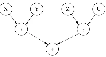
We would like our program to have several independent activities, each of which executes at its own pace.This is calledconcurrency.There should be no interference
X Y Z U
* *
+
Figure 1.3: A simple example of dataflow execution.
among the activities, unless the programmer decides that they need to communi-cate.This is how the real world works outside of the system.We would like to be able to do this inside the system as well.
We introduce concurrency by creating threads.A thread is simply an executing program like the functions we saw before.The difference is that a program can have more than one thread.Threads are created with thethread instruction.Do you remember how slow the originalPascalfunction was? We can callPascalinside its own thread.This means that it will not keep other calculations from continuing. They may slow down, ifPascalreally has a lot of work to do.This is because the threads share the same underlying computer.But none of the threads will stop. Here is an example:
thread P in P={Pascal 30} {Browse P} end
{Browse 99*99}
This creates a new thread.Inside this new thread, we call{Pascal 30}and then callBrowseto display the result.The new thread has a lot of work to do.But this does not keep the system from displaying99*99immediately.
1.11
Dataflow
declare X in
thread {Delay 10000} X=99 end {Browse start} {Browse X*X}
The multiplication X*X waits until X is bound.The first Browse immediately displays start.The second Browse waits for the multiplication, so it displays nothing yet.The {Delay 10000}call pauses for 10000 ms (i.e., 10 seconds). X is bound only after the delay continues.When X is bound, then the multiplication continues and the second browse displays 9801.The two operationsX=99 andX*X can be done in any order with any kind of delay; dataflow execution will always give the same result.The only effect a delay can have is to slow things down.For example:
declare X in
thread {Browse start} {Browse X*X} end {Delay 10000} X=99
This behaves exactly as before: the browser displays 9801 after 10 seconds.This illustrates two nice properties of dataflow.First, calculations work correctly in-dependent of how they are partitioned between threads.Second, calculations are patient: they do not signal errors, but simply wait.
Adding threads and delays to a program can radically change a program’s ap-pearance.But as long as the same operations are invoked with the same arguments, it does not change the program’s results at all.This is the key property of dataflow concurrency.This is why dataflow concurrency gives most of the advantages of concurrency without the complexities that are usually associated with it.Dataflow concurrency is covered in chapter 4.
1.12
Explicit state
How can we let a function learn from its past? That is, we would like the function to have some kind of internal memory, which helps it do its job.Memory is needed for functions that can change their behavior and learn from their past.This kind of memory is called explicit state.Just like for concurrency, explicit state models an essential aspect of how the real world works.We would like to be able to do this in the system as well.Later in the book we will see deeper reasons for having explicit state (see chapter 6).For now, let us just see how it works.
For example, we would like to see how often theFastPascalfunction is used.Is there some wayFastPascalcan remember how many times it was called? We can do this by adding explicit state.
A memory cell