Fithra Faisal Hastiadi

Regionalism in East Asia: The Role of North East Asian Nations

Fithra Faisal Hastiadi

PhD Candidate

Waseda University, Graduate School of Asia-Pacific Studies fithra@asagi.waseda.jp; fithra_faisal@yahoo.com

Abstract

Regionalism has now become a very popular phrase since this action has taken place into every inch of the World, East Asian region is no exception. For the past few years, regionalism has been progressing in East Asia in the form of Free Trade Agreements (FTAs) and Economic Partnership Agreements (EPAs). The likes of China, Japan, and Korea (CJK) as the economic front runners are regarded to be the key actors in stimulating regional economic growth through some opulent trade agreements. In this sense, the triangular trade agreement between CJK will become a significant ingredient that can cope with the necessary condition that is to create East Asian welfare. Unfortunately, with the absence of such agreements, the present intra regional trade scheme in CJK is not sufficient to meet the target. This paper uncovers the inefficient scheme through Engle-Granger Cointegration and Error Correction Mechanism. Moreover, the paper underlines the importance of triangular trade agreement for accelerating the phase of growth in the region. This agreement will then provide a major boost in the form of spillover effect for the ASEAN4 which represent South East Asian Region. Employing Two Stage Least Squares (2SLS) in a static panel fixed effect model, the paper argues that the spillover effect will function as an impetus for creating region-wide FTA. Furthermore, the paper also identifies a number of economic and political factors that can support the formation of East Asian Regionalism in the long run.

Key words: Regionalism, Engle-Granger Cointegration, Error Correction Mechanism, Fixed Effect, Two Stage Least Squares

JEL: F15, C13, C22, C33

A.Introduction

In this new millennium, regionalism has begun to emerge in East Asia. East Asian Countries have been focusing on ways to expand intra regional trade that include: the establishment of Regional Trade Agreements (RTAs) in the form of Free Trade Agreements (FTAs) and Economic Partnership Agreements (EPAs). The trend towards regionalism has created a profound regional and indeed global significance (Harvey and Lee, 2002). Japan, Korea and China are regarded as the key actors for such action in East Asia.

Being acknowledged as the economic front runners, Japan, China and Korea are assumed to have heavy responsibility for the economic welfare in the East Asian region. It is very obvious that East Asian regionalism cannot be put into practice without these countries’ strong support. Unfortunately, the lack of institutional arrangements among these giant countries has stalled the overall welfare effect for the East Asian communities. The present driving force of the China-Japan-Korea (CJK) relationship is the market by which in some sense is not enough; it should be matched by regionalism. The main focus of the regionalism is to make these countries grow together so that it can spread positive externalities throughout the East Asian region. In the long run it is expected that CJK will lead regionalism in East Asia.

The structure of this paper proceeds as follows. The first section studies the economic structures and trade patterns in the CJK. The next section examines the effect of openness in the CJK to economic growth in these particular countries. The third section analyzes the prospects of the CJK increased welfare in creating spillover effect to ASEAN4, which in this paper serves as a proxy for ASEAN countries. The last section presents the future trend and path towards East Asian Regionalism.

B.Japan, China and Korea Economic Relation

transformation of trade structures. In the early 90’s, primary commodities accounted for more than one third of China’s total export to Japan and Korea. In this new millennium, it is still top Chinese export to Japan and Korea, but it is persistently followed by the fast growth of machinery and transport (Chan and Chin Kuo, 2005). From this point of view, trade within the north East Asian region is deemed to have substantial movement as a result from the shift of trade towards a more industrialized structure. The emergence of China as a regional manufacturing center is a dominant factor that contributes the trade shift.

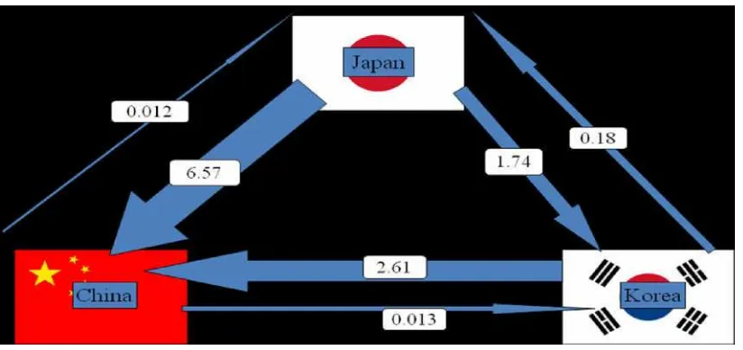
The overall picture of the trade amongst these countries is described in figure 1. It is clear that trade activity is very intense by which performs as the major contributing factor for economic growth in the region. The vast amount of trade has been very likely steered up by the amount of FDI flows among them with Japan as the sole leader of it (figure 2). In other words, the creation of economic transformation in China and Korea that geared up the trade was enchanted by Japan’s role in making investment in those countries.

Figure 1.Trade among Japan, China and Korea(2006, $billion)

Source: Watanabe (2008)

Figure 2.Investment among Japan, China and Korea(2005, $bilion)

Source: Watanabe (2008)

B.1. Measuring the short and the long run equilibrium of export to GDP

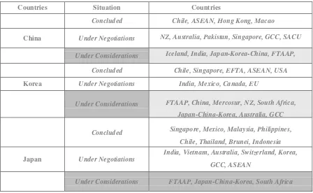
As already explained earlier, Japan, China and Korea are experiencing golden period in doing export among them. Economic welfare is the most notable goal which links in this activity, but is it sufficient to boost the economy in the long run? A pure market driven activity without specific regional trade agreement might sometime create bias. It is clear that Japan, Korea and China are lacking of such agreement among them (Urata and Kiyota, 2003) as described in the table 1.

Table 1. Japan, China and Korea FTAs/EPAs

Source: Japanese Ministry of Economy, Trade and Industry, 2007

To make an effective regionalism, Japan, China and Korea should support each other. Therefore, intra regional cooperation within the CJK must take place by which can create sustainable growth in East Asian region. The following sections serve to prove export sustainability to economic growth, in the absence of trade arrangements, for the short and the long run. Engle-Granger Cointegration and Error Correction Mechanism1 test are then employed for this cause.

B.1.1. Defining the Long Run Equilibrium: Engle Granger Cointegration Test

In doing Engle Granger Cointegration test, this paper divides the export relationship in to three parts which are described in the following equations:

i. China and Japan Export Relationship

(1) (2) ii. Korea and Japan Export Relationship

(3) (4)

1This test employs time series quarterly data of GDP and for Japan, China and Korea ranging from 1985 to 2004. The data is taken from CEIC database

Countries Situation Countries

Concluded Chile, ASEAN, Hong Kong, Macao

China Under Negotiations NZ, Australia, Pakistan, Singapore, GCC, SACU

Under Considerations Iceland, India, Japan-Korea-China, FTAAP, Switzerland

Concluded Chile, Singapore, EFTA, ASEAN, USA Korea Under Negotiations India, Mexico, Canada, EU

Under Considerations FTAAP, China, Mercosur, NZ, South Africa, Japan-China-Korea, Australia, GCC

Concluded Singapore, Mexico, Malaysia, Philippines, Chile, Thailand, Brunei, Indonesia

Japan Under Negotiations

India, Vietnam, Australia, Switzerland, Korea, GCC, ASEAN

iii.China and Korea Export Relationship

(5) (6)

In these equations, JPGDP, CHGDP and KRGDP are Japan’s GDP, China’s GDP, and Korea’s GDP respectively while Export JP, Export CH and Export KR are the variables of export destinations to Japan, China and Korea. It would be possible to cointegrate Export and GDP since the trend in export and GDP would offset to each other, creating a stationary residual. The residual is called a cointegration parameter. In the data, if we find that the initial regression of the residual (ut) gives stationarity it means that ut is stationary at order 0 (level) and it is notated as I(0). But ifutis stationer in first difference, the variables of Export and GDP will be cointegrated in the first difference which can be notated with I(1).

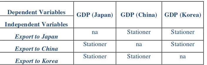
Table 2. Cointegration Parameters

Dependent Variables

Independent Variables

GDP (Japan) GDP (China) GDP (Korea)

Export to Japan na Stationer Stationer

Export to China Stationer na Stationer

Export to Korea Stationer Stationer na

From table 2 we can see that, GDP and export relationship in the CJK yields stability in the long run. It is proven by the stationarity of the error term in each of the cases. The cointegration test that proves long run equilibrium describes that the model is not spurious. Export is proven to be the engine of economic advancement in these countries. It approves some previous research as the likes of Heller and Porter (1978), Feder (1983), Ram (1985), Dorasami (1996), Ghatak, Subrata, Milner, Utkulu (1997) and Ekanayake (1999) of export and economic growth relationship.

B.1.2 Defining the Short Run Equilibrium: Error Correction Model

We have seen the long run relationship between Export and GDP. However, in order to make it objective, we should also see the short run since it is still plausible to perceive disequilibrium. Thus,

could be noted as equilibrium error. This error then could

be used to relate the behavior of the short run Japanese GDP The technique to correct short-run disequilibrium to its long run long run equilibrium is called Error Correction Mechanism (ECM). The model of ECM is as follows:

(7) is a cointegrated error lag 1, or could be noted mathematically as:

(8)

In this equation, is the difference in GDP for Japan, Korea and China, while is the difference in export from country X to Country Y. As for example,

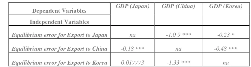
Table 3. Equilibrium Errors Dependent Variables

Independent Variables

GDP (Japan) GDP (China) GDP (Korea)

Equilibrium error for Export to Japan na -1.0 9 *** -0.23 *

Equilibrium error for Export to China -0.18 *** na -0.48 ***

Equilibrium error for Export to Korea 0.017773 -1.33 *** na Note: Statistical significance is indicated by *(10%), **(5%), and ***(1%)

i.Japan

In the short run, there is an equilibrium error for Japan’s Export to China with its relation to Japan’s GDP. The coefficient of residual gives negative sign (-0.18), which means that Japan’s Export to China is below the long run equilibrium. This will only lead to a rise of export for the following periods. But it is important to note that the absolute value of the coefficient (adjustment rate) is very small (0.18). This suggests that Japan’s Export to China is moving in a slow phase to reach the long run equilibrium.

As for the relationship between Japan and Korea, the equilibrium error of the export trend is not significant. These suggest that Japan’s GDP is adjusting to the change in Japan’s export to Korea in the same period of time. In other words, Japan and Korea relationship in terms of export has already reached steady state level.

ii.China

The residuals for the relationship between China’s GDP with China’s Export to Japan and Korea are significant. These suggest that there is an equilibrium error in the short run. The negative signs put the Export for a constant rise to reach the long run equilibrium. In China’s case, the adjustment rate or the phase of acceleration for the long run equilibrium is very fast. It can be seen through the absolute value of the equilibrium error coefficients which are 1.09 and 1.33 for China’s relationship to Korea and Japan respectively.

iii. Korea

Korea’s case is somewhat similar to China. The residuals for the relationship between Korea’s GDP with Korea’s Export to Japan and China are significant. It yields similar explanation with China’s case. However, the adjustment rate for the case of Korea is slower than China’s but it is still faster than Japan’s. It gives the absolute value of 0.23 and 0.48 for Korea’s trade relationship to Japan and China respectively.

B.1.3. Interim conclusion

From the ECM, we can conclude that North East Asian region is not moving at the same phase to reach the long run equilibrium, which in this case Japan is the slowest one. The insignificant value of acceleration rate for the case of Japan trade relationship with Korea is also important point to note since it can be interpreted as an exhausted Korean market for Japanese products (steady state condition). These facts are very crucial since it diminishes Japan’s role as the sole leader in the north East Asia. Although whoever the leader is not to important, but the stalled effect of a country’s economic growth in these region will only serve as stumbling blocks in creating East Asian welfare. In order to strengthen regional welfare and accelerate the phase of adjusting, economic integration must take place.

C. The Openness in Trade

These countries may have aggressively reached other countries in making FTA’s and EPA’s but none of which have been progressing among them (see table 1). The reason of it will be a subject for another research, while this section tries to focus on the effect of such agreement2 to the economy. The lack of trade arrangements that liberalize the sector of economy is being noted as the main factor that contributes intra regional trade ineffectiveness in north East Asia. This hypothesis will be proved in the following sections to come.

C.1 Openness with customized RPL index

Export lead growth approach that has been done in the previous section with cointegration and error correction model has actually provided the basis to measure openness3 of a country, but in some ways this alone is not enough. It only works for confirming the paradigm of trade as an engine of growth but it is not sufficient to measure a more robust pattern of openness. Therefore, we then may have to address Dollar’s Relative Price Level (RPL index).

This index is a measure of outward orientation of an economy that is based on international comparisons of price levels compiled for 121 countries by Summers and Heston (1988). They price the same basket of consumption goods in domestic currency in different countries and then convert the measure into US dollars using the official exchange rate. Using the US as the benchmark country, the index of country i's relative price level (RPL) is:

RPLi = 100 XPi/PusX 1/e (10)

Where e is the exchange rate (no. of units of domestic currency per unit dollar) and Pi is the consumption price index for country i and Pus is the consumption price index for US. Hence, one could use cross-country variations in these price levels to measure inward- or outward-orientation resulting from trade policy. With using the same analogy, this paper then customizes the RPL index into this formula:

RPLi = 100 XPi/PtpX 1/e (11)

WherePtpis the consumption price index for the trading partner and e is the exchange rate (no. of units of domestic currency per unit of trading partner currency). The customized RPL is then become a powerful tool to analyze trade openness between the trading countries.

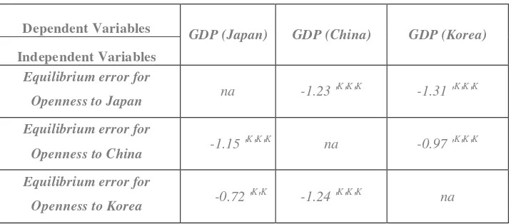
C.2 Error Correction Mechanism (ECM) of RPL index and GDP

As already explained in the previous section, ECM provides the description of short run shock. In this particular case4, we examine the openness vis a vis trade liberalization trend in north East Asia

region. (12)

This equation mimics equation 7, but the previous dependent variable is substituted from export to RPL in order to suit the goal which is to measure the openness. is the difference in GDP from Japan, Korea and China, is the difference in RPL from a country X to Country Y. measures the openness of trade from of country X towards Y. Below is the outputs for each country :

2 Regional trade agreement provides openness to some sectors of economy

3 Several cross-country studies investigating outward orientation and growth have used export growth as a proxy for outward orientation. The main examples of this approach are Michaely (1977), Heller and Porter (1978), Feder (1983), Ram (1985) and more recently Levin and Raut (1997).

Table 4. Cointegration Parameters

Note: Statistical significance is indicated by *(10%), **(5%), and ***(1%)

From this particular test we can see that generally trade openness is affecting a country’s GDP in a positive way. But in the short run, trade openness in the CJK is still below the equilibrium. This suggests that trade openness is still finding its form in this area. Although we might not see regionalism which liberalize trade in the short run, but the trend towards openness in trade vis a vis regionalism is progressing in a respectful manner. We can see this through the adjustment rate for the long run equilibrium (the coefficients of residuals) that yields an average of 1.1, consequently we might see regionalism in North East Asia happen in the future.

D. The Spillover Effect from Japan-Korea-China Triangular Trade to ASEAN 4

As giants of Asia, the growth of Japan, Korea and China will most likely create positive effect to the neighboring countries. Regionally speaking, the growth of North East Asia will boost the East Asian growth as whole, in this sense we might want to exercise its effect to ASEAN countries. To simplify things, this paper limits the effect to ASEAN4 since these countries have the same economic characteristics. This paper employs static panel data5 model for this purpose. The following sections provide the analysis.

D.1 Examining the spilover effect through panel data model

A static panel data model can be specified as follows:

Yit

=

X

it

β+λ

t

+η

i

+

ε

it t=1,...

,

T i=1,...

,

N

(13)

Where: λt and ηiare time and individual specific effects respectively,x itis a vector of the explanatory variables, (i) is the time component of the panel, (N) is the cross-section dimension (or the number of cross-section observations), and N x T is the total number of observations. The idea is to run the models in order to have a consistent estimator for the β coefficients, and the model (fixed or random) choice depends on the hypothesis assumed for the relationship between the error-term (εit) and the regressors (x it ). The static panel data analysis developed in the empirical section of the paper was based on two basic panel models, the fixed (FE) and the random (RE) effect models. Since the time periods (1989-2007) exceed the individual observations (Indonesia, Malaysia, Thailand, Philippines) therefore FE is considered as the most appropriate method (Nachrowi and Usman, 2008). The model is described as follows:

(14)

5 The panel data is analyzed annually from 1989 to 2007 which consist of ASEAN 4’s Export, Import, Consumption, Investment, Government expenditure, GDP, and GDP of Japan, China, Korea. The data is taken from WDI online database

.Where: Y

X

i t = In d e p e n d e n t V a r i a b l e s ( A S E A N 4 c o n s u mp t i o n g r o w t h , i n v e s t me n t g r o w t h , government expenditure growth, export-import growth and Japan-China-Korea6 GDP growth for time t)

Witand Zitare varible dummy which are defined as follows :

Wit =1 for country i, where i = Indonesia, Malaysia, Philippines, Thailand = 0 for others

Zit =1 for Period t where t = 1989, 1990..., 2007 = 0 for others

The above structural equation is actually a simultaneous equation7in which employs causality relationship. To see the simultaneity, the above model can be decomposed into four parts:

(15) (16)

(17) (18)

Equation 15 describes the effects of ASEAN 4 consumption (Ct), investment (It), government expenditure (Gt), export growth (Xt) and the North East Asian GDP growth (JGDPt, CGDPt, KGDPt) on ASEAN4 GDP growth (Yt). From the model, it is clear that consumption growth, investment growth and export growth have their own determinants that simultaneously form the structural equation. Consumption growth (Ct) is formed by last year’s consumption growth (Ct-1), and the present GDP growth (Yt), Investment (It) on the other hand is influenced by the interest rate (rt) and the GDP growth (Ct). It is also expected that exchange rate (EXt), consumption growth (Ct) and trading partners economic growth (JGDPt, CGDPt, KGDPt) have some influences on export growth (Xt) for ASEAN 4.

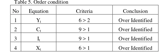
From the structural equation, we can divide the variables into two, endogenous and predetermined (exogenous). The first one is treated as stochastic while the latter as non stochastic. To see which simultaneous model that can satisfies the need, we have to address the identification process. If K is the number of exogenous variables within the model, k is the number of exogenous variables within the equation and M is the number of endogenous variable within the model, so the criteria to state whether an equation is unidentified, just identified, or over identified are describe as follows:

If K-k < M-1, so the equation is unidentified

If K-k = M-1, so the equation is exactly identified If K-k > M-1, so the equation is over identified

Based form the above criteria, table 5 summarize the order condition from the system: Table 5. Order condition

No Equation Criteria Conclusion

1 Yt 6 > 2 Over Identified

2 Ct 9 > 1 Over Identified

3 It 9 > 1 Over Identified

4 Xt 6 > 1 Over Identified

6 Japan, Korea and China GDP are included in the structural equation referring to Tran Van Hoa’s (2003) assessment in the model

7 The model is simultaneous because we cannot determine C, I, G,X, M or Y without knowing the other

9

assumes that there is a secondary predictor that is correlated to the problematic predictor but not with the error term. Given the existence of the instrument variable, 2SLS regression analysis uses the following two methods: In the first stage of the two-stage least squares 2SLS regression analysis, a new variable is created using the instrument. In the second stage of the 2SLS regression analysis, the model-estimated values from stage one are then used in place of the actual values of the problematic predictors to compute an OLS model for the response of interest. Below is the detailed procedure of 2SLS:

In stage one, least square regression on the reduced form equation has to take place by which it can yields Ct-1, Yt-1, rt, Gt, EXt, JGDPt, CGDPt, KGDPtas the instrumental variables, therefore all equations from 15 up to 18 have to be transformed into reduced form equation as the followings :

(19) (20) (21)

(22) Notes :

Notes

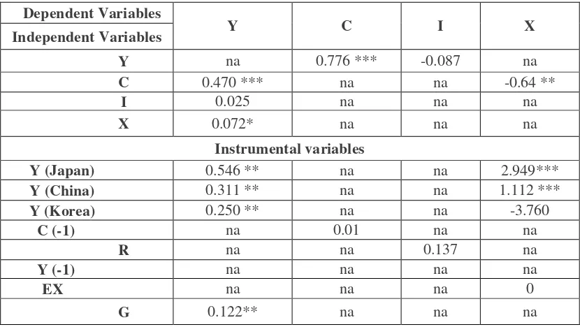
From stage one we get as the fitted values with which we can run for the secondstage. In stage two, these fitted values are then plugged in to the main equation. The last step is to run least squares on each of the above equations to get 2SLS estimation as described below in table 6.

Table 6. Two Stage Least Squares Regression Output :

Note: Statistical significance is indicated by *(10%), **(5%), and ***(1%)

8Two-stage least squares regression (2SLS) is a method of extending regression to cover models which violate ordinary least squares (OLS) regression's assumption of recursivity, specifically models where the researcher must assume that the

disturbance term of the dependent variable is correlated with the cause(s) of the independent variable(s)

From the output above we can conclude that the North East Asian (Japan, Korea and China) economic

Dependent Variables

Independent Variables Y C I X

Y na 0.776 *** -0.087 na

C 0.470 *** na na -0.64 **

I 0.025 na na na

X 0.072* na na na

Instrumental variables

Y (Japan) 0.546 ** na na 2.949***

Y (China) 0.311 ** na na 1.112 ***

Y (Korea) 0.250 ** na na -3.760

C (-1) na 0.01 na na

R na na 0.137 na

Y (-1) na na na na

EX na na na 0

growth boost the ASEAN4 economic growth, it confirms the proposition of this paper. Investment flows, in the form of FDI, has also operated as a dominant integrating power in East Asia as whole. Although we cannot find legitimate determinant for FDI9in the output, but it is clear that FDI is trade related in nature (Wong, 2004). With its essentially open and outward-looking economies, the region is highly dependent on foreign investment for its economic growth. But still, the boosting power is not as much as in the spillover effect from the giant countries of Japan, Korea and China. Japan, in terms of GDP growth, has the biggest influence towards ASEAN4 followed by China and Korea at the second and third place. This fact is described by the coefficient parameter that gives the value of 0.546, 0.311 and 0.250 for Japan, China and Korea respectively.

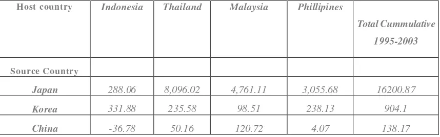
The ranking of influence is presumably caused by the number FDI inflows to ASEAN from these countries as described below in table 7. The only bias is on China and Korea, even though the cumulative FDI from Korea to ASEAN4 was bigger than China’s, but it does not seem to be reflected on the ranking of influence. As for this, it is assumed that the high economic growth rate of China had been the major contributing factor (Urata, 2008) that overtook the influence of Korea’s cumulative FDI flow to ASEAN4. However, such factor is not enough to surpass10 Japan’s influence to ASEAN4’s economic growth since Japan’s FDI contribution to ASEAN4 outweighed China’s by more than one hundred folds.

Table 7. FDI flows to ASEAN 4 (US$ million)

Host country Indonesia Thailand Malaysia Phillipines

Total Cummulative 1995-2003

Source Country

Japan 288.06 8,096.02 4,761.11 3,055.68 16200.87

Korea 331.88 235.58 98.51 238.13 904.1

China -36.78 50.16 120.72 4.07 138.17

Source: ASEAN secretariat

The story goes hand in hand with the flying-geese hypothesis that was developed by Japanese economist, Kaname Akamatsu (1935). This model has beeen frequently proposed to examine the patterns and characteristics of East Asian economic integration. The premise of the flying-geese pattern suggests that a group of nations in this region are flying together in layers with Japan at the front layer (Xing, 2007). The layers signify the different stages of economic development achieved in various countries. In the flying-geese model of regional economic development, Japan as the leading goose leads the second-tier geese (China, Korea) which, in their turn, are followed by the third-tier geese (ASEAN4).

Another important thing to note is the low significant value of exports within ASEAN4 in terms of creating GDP growth. These are intriguing facts since export is considered as the main determinant of GDP growth. It is suspected that the effect of rivalry between ASEAN4 members and China is the main factor which creates insignificant value. This factor is supported by Roland-Host and Weiss (2004) that pointed out China’s emergence for creating short and medium term direct and indirect competition between ASEAN and China. They argued that ASEAN and China are experiencing intensified export competition in prominent third markets. This can lead to painful domestic structural adjustments within the ASEAN in the short run. Then again the mind set in viewing the economic opportunity or threat depends on whether China’s economy is perceived as complementary or competitive

9 it is described by the insignificant value of interest rate and GDP growth towards investment (table 6)

10 From the ECM simulation as confirmed earlier, we found that China has taken over Japan’s role in East Asia. But this is true if we address the long run effect. This section only measures the present condition in the absence of the intertemporal problem

11 opportunities and overcome the competitive threats.

Chia (2006) argued that the differences in resource and factor endowments, production structures, and productivities lead to a complementary relationship, whereas similarities in these areas lead to a competitive relationship. Data from the rapidly growing intra-industry trade in electronic products and components shows that at high levels of disaggregation, product differentiation creates complementarity in production and trade. Even in non manufactures such complementarity can be found: fruits and vegetables produced in China’s temperate region are complementary to those produced in ASEAN’s tropical region. In the long run, regionalism is expected to accommodate welfare for East Asia. The growing significance of China market for ASEAN will serve as the basis for regionalism. Thus, a unified East Asia could accelerate the momentum of overall trade liberalization and boost regional economic growth.

E. The Future Trend of East Asian Regionalism (EAR)

The next task is to shape the future of EAR, but then will the future exist? In part C of this paper, we measure the trend toward openness vis a vis regionalism by using ECM for the RPL index in North East Asia (CJK). Since we include two sub regions, the best way to measure it is by using test of convergence of the term of trade for CJK and ASEAN4. The notion of convergence implies that differences between the series must follow a stationary process (Bernard & Durlauf, 1996; Oxley & Greasley, 1995). Thus, stochastic convergence implies that income differences among countries cannot contain unit roots.

Following Bernard and Durlauf (1995), stochastic convergence occurs if the differential log trade system, yt, follows

a stationary process, where = , where is the logarithm term of

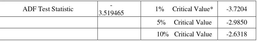
trade of ASEAN4, and is logarithm term of trade of CJK, and both series are in the first difference (I(1)). Stochastic convergence is tested by using the conventional augmented Dickey-Fuller (ADF) regression which shows a significance result in proving stationarity for (see Table 8). This indicates long-run convergence between the two trading systems.

Table 8. ADF Test for Term of Trade

ADF Test Statistic

-3.519465 1% Critical Value* -3.7204 5% Critical Value -2.9850 10% Critical Value -2.6318 *MacKinnon critical values for rejection of hypothesis of a unit root.

A major drawback of the standard ADF unit root test procedure is that the power of the test is quite low. To overcome this problem, the paper utilizes cointegration test as suggested by Baharumshah et al. (2007). The following is the Engle Granger Cointegration:

(23)

Table 9. ADF Test for Cointegration Residual

ADF Test Statistic -5.623714 1% Critical Value* -3.7204 5% Critical Value -2.9850 10% Critical Value -2.6318 *MacKinnon critical values for rejection of hypothesis of a unit root.

F. Factors Contributing to EAR

Feng and Genna (2003) argued that the formation of an economic union requires that the homogeneity of domestic economic institutions and the process of regional integration reinforce each other. Economic institutions in this context are represented by inflation, taxation, government regulation. Another variable that might enhance integration is population as already identified by Tamura (1995). He then argued that due the agglomeration economy, the larger the region’s population, the greater the incentive to integrate the region into a larger market. Scholars like Milner and Kubota (2005) even pointed out democracy as an important factor that could foster regionalism. Their empirical work on the developing countries from 1970-1999 showed that regime change toward democracy was associated with trade liberalization, and regionalization.

Given those works, this paper tries to combine the variables into one complete model that can determine the formation of EAR. The formula as follows:

(20)

Where:

Openit = Regionalism for time t and country i

Xit = Independent Variables (ASEAN4 + CJK’s log(road), tax, democracy, governance, log(industry), telephone, inflation, log(population))

Witand Zitare varible dummy which are defined as follows :

Wit =1 for country i, where i = Indonesia, Malaysia, Philippines, Thailand = 0 for others

Zit =1 for Period t where t = 1989, 1990..., 2007 = 0 for others

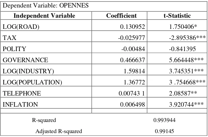
13 Table 10. Factors Affecting Openness

Dependent Variable: OPENNES

Independent Variable Coefficient t-Statistic

LOG(ROAD) 0.130952 1.750406*

TAX -0.025977 -2.895386***

POLITY -0.00484 -0.841395

GOVERNANCE 0.466637 5.664448***

LOG(INDUSTRY) 1.59814 3.745351***

LOG(POPULATION) 1.36772 3 .754668***

TELEPHONE 0.00743 1 2.08587**

INFLATION 0.006498 3.920744***

R-squared 0.993944

Adjusted R-squared 0.99145

Note: Statistical significance is indicated by *(10%), **(5%), and ***(1%)

The results shows us that Economic and political factors such as Infrastructure (road and telephone), Governance, Taxation policy, Industrialization and Inflation have significant effect towards Regionalism (Openness) in East Asia while Democracy (Polity) plays insignificant role. The signs of coefficient for road, telephone, governance, tax, inflation and industrialization are positive which mean the bigger the variable the more they create Openness. The negative sign of the coefficient for tax describes the opposite relation between corporate tax rate and the future prospect of EAR, the higher the rate the more it will the deteriorate the EAR

E. Conclusion

We have made an interim conclusion that export leads the overall growth in North East Asia. However, it is important to note that Japan’s phase of adjustment towards long run equilibrium is quite slow compared to the likes of Korea and China. This only yields as a stumbling block in forming regionalism in East Asia. The hard task is about making these countries move together in the same phase, which is why regionalism has to take place.

Since regionalism is an abstract term, the use of RPL index is essential. RPL index is a proxy of outward orientation of a country or in other words it is a representation of regionalism. Regionalism in this case goes hand in hand with openness in which it creates trade arrangements that liberalize some sectors in the economy. The ECM simulation gives a clear picture of the current form of openness which is below the equilibrium. It suggests that the trend towards regionalism is still far behind. It somewhat confirms the ineffectiveness of current triangular trade in North East Asia. It is expected that regionalism can eliminates such bias in trade.

Moreover, since North East Asian countries has a big scale of economy, its economic development will substantially affect the neighboring countries in East Asia specifically ASEAN4. It is demonstrated by the large share of China-Japan-Korea growth that affects ASEAN4’s GDP.

The growing significance11of China, Japan and Korea market for ASEAN4 will then serve as the basis for a single East Asian Wide FTA. The next task is to shape the future of EAR, but then will the future exist? Using the test of convergence, it is found that EAR will be there to stay. The robust finding surely creates optimistic view for EAR. But knowing the future is not enough, we still need to find out the clear path to reach the future. What are the paths then? From a static panel data simulation it is found that sound physical infrastructure, good governance, inflation, competitive taxation policy, sizeable market and the trend towards industrialization are the main factors that serve as building blocks for EAR.

To wrap up, EAR will enable the region to cope with the future challenges of globalization and remain internationally competitive. An integrated East Asia would lead to the advancement in economies of scale, fuller development of production networks. Moreover, Chia (2007) stated that EAR could hold close the less developed East Asian economies which would otherwise become marginalized as they lack the attraction of sizeable market and lack negotiating resources.

11 It is shown from table 6 at export and import column equation in which ASEAN 4 trade tends to rely on the market size in North East Asia (Japan, Korea and China)

REFERENCES

Akamatsu, Kaname, 1935. Wagakuni yomo kogyohin no susei [Trend of Japanese Trade in Woolen Goods], Shogyo Keizai Ronso [Journal of Nagoya Higher Commercial School] 13: 129-212.

Angrist, J. D, & Imbens, G. W, 1995. Two-stage least squares estimation of average causal effects in models with variable treatment intensity. Journal of the American Statistical Association, 90(430), 431-442

Arellano, M, 1995. On the testing of correlated effects with panel data", Journal of Econometrics, 59, 87--97.

Chan, Sarah and Chun-Chien Kuo, 2005. Trilateral Trade Relations among China, Japan and South Korea:Challenges and Prospects of Regional Economic Integration, East Asia, Vol. 22, No. 1, pp. 33-50.

Chia, Siow Yue, 2006. ASEAN-China Economic Competition and Free Trade Area, Asian Economic Papers The Earth Institute at Columbia University and the Massachusetts Institute of Technology, 2007. Challenges and Configurations of a Region-wide FTA in East Asia, FONDAD Conference.

Cohen, Benjamin J, 1997. The Political Economy of Currency Regions, in Helen Milner and Edward Mansfield (eds) The Political Economy of Regionalism, New York: Columbia University Press. Debraj, Ray, 1998. Development Economics. Princeton University Press, New Jersey.

Dollar, David, 1992. Outward Oriented Developing Economies Really Do Grow More Rapidly: Evidence From 95 LDCs, 1976-85, Economic Development and Cultural Change, Vol. 4 No. 3, 523-544. Doraisami, Anita. 1996. Export Growth and Economic Growth: A Reexamination of Some Time-Series Evidence of the Malaysian Experience , The Journal of Developing Areas.

Ekanayake, E.M, 1999. Export and Economic Growth in Asian Developing Countries: Cointegration and Error-Correction Models, Journal of Economic Development.

Engle, R.F. and C.W.J. Granger, 1987. Cointegration and Error Correction: Representation, Estimation and Testing, Econometrica, 55, March, 251-76.

Feder, G, 1983. On Export and Economic Growth, Journal of Development Economics, 5, 59-73.

Feng, Yi and Gaspare M. Genna, 2003. Regional integration and domestic institutional homogeneity: a comparative analysis of regional integration in the Americas, Pacific Asia and Western Europe, Review of International Political Economy, Routledge.

15

Evidence for Malaysia, Applied Economics, 29, 2 13-223. Gujarati, Damodar N, 1995. Basic Econometrics, 3rd edition. Singapore: McGraw-Hill inc.

Harrison, Ann, 1996. Openness and Growth: A Time Series, Cross Country Analysis for Developing Countries, Journal of Development Economics, Vol.48 No.2, March, 419-447.

Harvie, Charles and Hyun Hoon Lee, 2002. New Regionalism in East Asia: How Does It Relate to the East Asian Economic Development Model, University of Wollongong Department of Economics, Working Paper Series.

Heller, P.S. and R.C. Porter, 1978. Export and Growth: An Empirical Reinvestigation, Journal of Development Economics, 5, 191-193.

Hoa, Tran Van, 2003. New Asian Regionalism: Evidence on ASEAN+ 3 Free Trade Agreement From Extended Gravity Theory and New Modeling Approach, University of Wollongong, Economics Working Paper Series.

Kaufmann, Daniel, Aart Kraay and Massimo Mastruzzi, 2003. Governance Matters III: Governance Indicators for 1996-2002, World Bank Policy Research Department Working Paper.

Kawai, Masahiro, 2005. East Asian economic regionalism: progress and challenges, Journal of Asian Economics, Elsevier.

Kawai, Masahiro and Ganeshan Wignaraja, 2007. Regionalism as an Engine of Multilateralism: A Case for a Single East Asian FTA. ADB Working Paper series on Regional Economic Integration no.14. Love, Jim and Ramesh Chandra, 2004. An Index of Openness and its Relationship With Growth in India, The Journal of Developing Areas.

Michaely, M, 1977. Export and Growth: An Empirical Investigation, Journal of Development Economics, 4, 49-53.

Milner Helen V and Keiko Kubota, 2005. Why the Move to Free Trade? Democracy and Trade Policy in the Developing Countries, International Organization, Vol. 59, No. 1, pp. 107-143, Cambridge University Press.

Nachrowi,Djalal, 2007. Ekonometrika Untuk Analisa Ekonomi dan Keuangan [Econometrics for Economic and financial analysis], Faculty of Economics University of Indonesia.

Ram, Rati, 1985. Export and Economic Growth: Some Additional Evidence, Economic Development and Cultural Change, Vol.33 No.2, January, 415-425.

Roland –Holst, David and John Weiss, 2004. ASEAN and China: Export Rival or Partners in Regional Growth? Blackwell Publishing Ltd.

Summers, R. and A. Heston, 1988. A New Set of International Comparisons of Real Product and Price Levels: Estimates for 130 Countries, 1950-1985, Review of Income and Wealth, March, 34, 1-25. Stubbs, Richard, 2002. ASEAN PLUS Three emerging East Asian Regionalism, University of California Press.

Tamura, Robert, 1995. Regional economies and market integration, Journal of Economic Dynamics and Control, Elsevier.

Urata, Shujiro and Kozo Kiyota, 2003. The Impacts of an East Asia Free Trade Agreement on Foreign Trade in East Asia, NBER Working Paper Series 10173 (December), National Bureau of Economic Research, Cambridge.

Yoshida, Tadahiro, 2004. East Asian Regionalism and Japan, Institute of Developing Economies, Jetro. Watanabe,

Yorizumi, 2008. Economic Partnership Agreement (EPA) of Japan and Economic Integration in Northeast Asia, Academic presentation, Graduate School of Media and Governance, Keio University.

Wong, John, 2004. China’s Economic Rise: Implications for East Asian growth and Integration, Bulletin on Asia-Pacific Perspectives.