Mathematics Tom M Apostol Calculus vol. 2

(1)

Tom

Apostol

CALCULUS

VOLUME II

ti Variable Calculus and Linear

Algebra, with Applications to

tial Equations and Probability

SECOND EDITION

John Wiley

Sons

(2)

George Springer,

Indiana University

(3)

To

(4)

(5)

PREFACE

This book is a continuation of the author’s Calculus, Volume Second Edition. The present volume has been written with the same underlying philosophy that prevailed in the first. Sound training in technique is combined with a strong theoretical development. Every effort has been made to convey the spirit of modern mathematics without undue emphasis on formalization. As in Volume I, historical remarks are included to give the student a sense of participation in the evolution of ideas.

The second volume is divided into three parts, entitled Linear Analysis, Nonlinear and Special Topics. The last two chapters of Volume I have been repeated as the first two chapters of Volume II so that all the material on linear algebra will be complete in one volume.

Part 1 contains an introduction to linear algebra, including linear transformations, matrices, determinants, eigenvalues, and quadratic forms. Applications are given to analysis, in particular to the study of linear differential equations. Systems of differential equations are treated with the help of matrix calculus. Existence and uniqueness theorems are proved by method of successive approximations, which is also cast in the language of contraction operators.

Part 2 discusses the calculus of functions of several variables. Differential calculus is unified and simplified with the aid of linear algebra. It includes chain rules for scalar and vector fields, and applications to partial differential equations and extremum problems. Integral calculus includes line integrals, multiple integrals, and surface integrals, with applications to vector analysis. Here the treatment is along more or less classical lines and does not include a formal development of differential forms.

The special topics treated in Part 3 are Probability and Numerical Analysis. The material on probability is divided into two chapters, one dealing with finite or countably infinite sample spaces; the other with uncountable sample spaces, random variables, and dis-tribution functions. The use of the calculus is illustrated in the study of both one- and two-dimensional random variables.

(6)

There is ample material in this volume for a full year’s course meeting three or four times per week. It presupposes a knowledge of one-variable calculus as covered in most first-year calculus courses. The author has taught this material in a course with two lectures and two recitation periods per week, allowing about ten weeks for each part and omitting the starred sections.

This second volume has been planned so that many chapters can be omitted for a variety of shorter courses. For example, the last chapter of each part can be skipped without disrupting the continuity of the presentation. Part 1 by itself provides material for a com-bined course in linear algebra and ordinary differential equations. The individual instructor can choose topics to suit his needs and preferences by consulting the diagram on the next page which shows the logical interdependence of the chapters.

Once again I acknowledge with pleasure the assistance of many friends and colleagues. In preparing the second edition I received valuable help from Professors Herbert S. Zuckerman of the University of Washington, and Basil Gordon of the University of California, Los Angeles, each of whom suggested a number of improvements. Thanks are also due to the staff of Blaisdell Publishing Company for their assistance and cooperation.

As before, it gives me special pleasure to express my gratitude to my wife for the many ways in which she has contributed. In grateful acknowledgement I happily dedicate this book to her.

T. M. A. Pasadena, California

(7)

Logical Interdependence of the Chapters ix

LINEA R S PA C ES

6

LINEA R I

T R A N S FO R M A T I O N S AND M ATRICES

D ET ER M I N A N T S

DIFFERENTIAL EQ UA TIO N S

4 EI G EN V A L U ES

, I A N D

EIG EN V ECTO RS SYSTEM S OF

DIFFERENTIAL EQ UA TIO N S

INTRODUCTION TO NUM ERICAL

A N A LY S I S

10 13

DIFFERENTIAL

H

LINE SET FUNCTIONS

CA LCULUS OF I N T EG R A L S AND ELEM ENTARY

SCA LA R A ND PROBABILITY

VECTOR FIELDS

OPERATORS ACTING ON EUCLIDEA N

S PA C ES 9

A PPLIC A T IO N S O F DIFFERENTIAL

C A L C U L U S

PROBA BILITI ES

(8)

(9)

PART 1. LINEAR ANALYSIS

1. LINEAR SPACES

1.1 Introduction

1.2 The definition of a linear space 1.3 Examples of linear spaces

1.4 Elementary consequences of the axioms 1.5 Exercises

1.6 Subspaces of a linear space

1.7 Dependent and independent sets in a linear space 1.8 Bases and dimension

1.14 Construction of orthogonal sets. The Gram-Schmidt process 1.15 Orthogonal complements. Projections

1.16 Best approximation of elements in a Euclidean space by elements in a

(10)

2.4 Exercises

2.11 Construction of a matrix representation in diagonal form 2.12 Exercises

2.13 Linear spaces of matrices

2.14 Tsomorphism between linear transformations and matrices 2.15 Multiplication of matrices

3.2 Motivation for the choice of axioms for a determinant function 3.3 A set of axioms for a determinant function

3.4 Computation of determinants 3.5 The uniqueness theorem 3.6 Exercises

3.7 The product formula for determinants

3.8 The determinant of the inverse of a nonsingular matrix 3.9 Determinants and independence of vectors

3.10 The determinant of a block-diagonal matrix 3.11 Exercises

(11)

Contents . . .

4. EIGENVALUES AND EIGENVECTORS

4.1 Linear transformations with diagonal matrix representations

4.2 Eigenvectors and eigenvalues of a linear transformation

4.3 Linear independence of eigenvectors corresponding to distinct eigenvalues

4.4 Exercises

4.5 The finite-dimensional case. Characteristic polynomials

4.6 Calculation of eigenvalues and eigenvectors in the finite-dimensional case

4.7 Trace of a matrix

4.8 Exercises

4.9 Matrices representing the same linear transformation. Similar matrices

4.10 Exercises

5.3 Eigenvalues and eigenvectors of Hermitian and skew-Hermitian operators

5.4 Orthogonality of eigenvectors corresponding to distinct eigenvalues

5.5 Exercises

5.6 Existence of an orthonormal set of eigenvectors for Hermitian and

114

5.7 Matrix representations for Hermitian and skew-Hermitian operators

5.8 Hermitian and skew-Hermitian matrices. The

of a matrix

5.9 Diagonalization of a Hermitian or skew-Hermitian matrix

5.10 Unitary matrices. Orthogonal matrices

5.11 Exercises

5.12 Quadratic forms

5.13 Reduction of a real quadratic form to a diagonal form

5.14 Applications to analytic geometry

5.15 Exercises

Eigenvalues of a symmetric transformation obtained as values of its

quadratic form

(12)

6. LINEAR DIFFERENTIAL EQUATIONS

6.1 Historical introduction

6.2 Review of results concerning linear equations of first and second orders 6.3 Exercises

6.4 Linear differential equations of order 6.5 The existence-uniqueness theorem

6.6 The dimension of the solution space of a homogeneous linear equation 6.7 The algebra of constant-coefficient operators

6.8 Determination of a basis of solutions for linear equations with constant coefficients by factorization of operators

6.9 Exercises

6.10 The relation between the homogeneous and nonhomogeneous equations 6.11 Determination of a particular solution of the nonhomogeneous equation.

The method of variation of parameters

6.12 Nonsingularity of the Wronskian matrix of

n

independent solutions of a homogeneous linear equation

6.13 Special methods for determining a particular solution of the nonhomogeneous equation. Reduction to a system of first-order linear equations

6.14 The annihilator method for determining a particular solution of the nonhomogeneous equation

6.15 Exercises

6.16 Miscellaneous exercises on linear differential equations 6.17 Linear equations of second order with analytic coefficients 6.18 The Legendre equation

6.19 The Legendre polynomials

6.20 Rodrigues’ formula for the Legendre polynomials 6.21 Exercises

7.3 Infinite series of matrices. Norms of matrices 194

(13)

Contents x v

7.6 The differential equation satisfied by

7.7 Uniqueness theorem for the matrix differential equation = 7.8 The law of exponents for exponential matrices

7.9 Existence and uniqueness theorems for homogeneous linear systems

198 199

with constant coefficients 200

7.10 The problem of calculating 201

7.11 The Cayley-Hamilton theorem 203

7.12 Exercises 205

7.13 Putzer’s method for calculating 205

7.14 Alternate methods for calculating in special cases 208

7.15 Exercises 211

7.16 Nonhomogeneous linear systems with constant coefficients 213

7.17 Exercises 215

7.18 The general linear system Y’(t) = P(t) Y(t) + Q(t) 217

7.19 A power-series method for solving homogeneous linear systems 220

7.20 Exercises 221

7.21 Proof of the existence theorem by the method of successive approximations 222 7.22 The method of successive approximations applied to first-order nonlinear systems 227 7.23 Proof of an existence-uniqueness theorem for first-order nonlinear systems 229

7.24 Exercises 230

Successive approximations and fixed points of operators 232

linear spaces 233

Contraction operators 234

Fixed-point theorem for contraction operators 235

Applications of the fixed-point theorem 237

PART 2. NONLINEAR ANALYSIS

Functions from to R”. Scalar and vector fields Open balls and open sets

Exercises

Limits and continuity Exercises

(14)

8.10 Directional derivatives and continuity 8.11 The total derivative

8.12 The gradient of a scalar field

8.13 A sufficient condition for differentiability 8.14 Exercises

8.15 A chain rule for derivatives of scalar fields

8.16 Applications to geometry. Level sets. Tangent planes 8.17 Exercises

8.18 Derivatives of vector fields 8. Differentiability implies continuity

8.20 The chain rule for derivatives of vector fields 8.21 Matrix form of the chain rule

8.22 Exercises

Sufficient conditions for the equality of mixed partial derivatives 8.24 Miscellaneous exercises

9.2 A first-order partial differential equation with constant coefficients 284

9.3 Exercises 286

9.4 The one-dimensional wave equation 288

9.5 Exercises 292

9.6 Derivatives of functions defined implicitly 294

9.7 Worked examples 298

9.8 Exercises 302

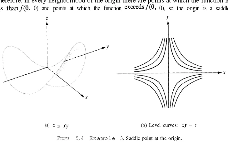
9.9 Maxima, minima, and saddle points 303

9. IO Second-order Taylor formula for scalar fields 308

9.11 The nature of a stationary point determined by the eigenvalues of the Hessian

matrix 310

9.12 Second-derivative test for extrema of functions of two variables 312

9.13 Exercises 313

9.14 Extrema with constraints. Lagrange’s multipliers 314

9. I5 Exercises 318

9.16 The extreme-value theorem for continuous scalar fields 319

9.17 The small-span theorem for continuous scalar fields (uniform continuity) 321

10. LINE INTEGRALS

10.1 Introduction

10.2 Paths and line integrals

(15)

Contents xvii

10.3 Other notations for line integrals 324

10.4 Basic properties of line integrals 326

10.5 Exercises 328

10.6 The concept of work as a line integral 328

10.7 Line integrals with respect to arc length 329

10.8 Further applications of line integrals 330

10.9 Exercises 331

10.10 Open connected sets. Independence of the path 332

10.11 The second fundamental theorem of calculus for line integrals 333

10.12 Applications to mechanics 335

10.13 Exercises 336

10.14 The first fundamental theorem of calculus for line integrals

10.15 Necessary and sufficient conditions for a vector field to be a gradient 339 10.16 Necessary conditions for a vector field to be a gradient 340

10.17 Special methods for constructing potential functions 342

10.18 Exercises 345

10.19 Applications to exact differential equations of first order 346

10.20 Exercises 349

10.21 Potential functions on convex sets 350

11. MULTIPLE INTEGRALS

11 Introduction 353

11.2 Partitions of rectangles. Step functions 353

11.3 The double integral of a step function 355

11.4 The definition of the double integral of a function defined and bounded on a rectangle

11.5 Upper and lower double integrals

11.6 Evaluation of a double integral by repeated one-dimensional integration 11.7 Geometric interpretation of the double integral as a volume

11.8 Worked examples 11.9 Exercises

11.10 Integrability of continuous functions

(16)

11.19 Green’s theorem in the plane

11.20 Some applications of Green’s theorem

11.21 A necessary and sufficient condition for a two-dimensional vector field to be a gradient

11.22 Exercises

Green’s theorem for multiply connected regions The winding number

1.25 Exercises

11.26 Change of variables in a double integral 11.27 Special cases of the transformation formula 11.28 Exercises

11.29 Proof of the transformation formula in a special case 11.30 Proof of the transformation formula in the general case 11.31 Extensions to higher dimensions

11.32 Change of variables in an n-fold integral 11.33 Worked examples

11.34 Exercises

12. SURFACE INTEGRALS

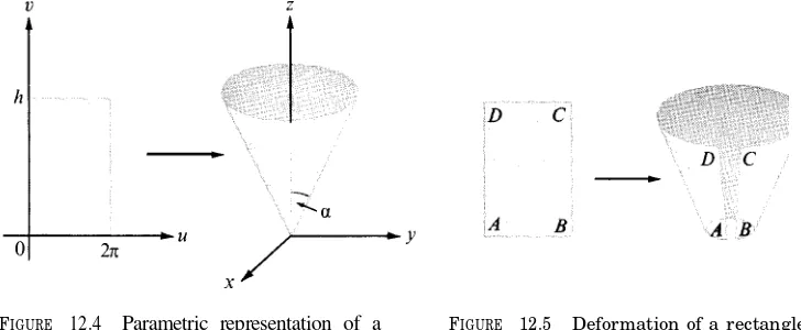
12.1 Parametric representation of a surface

12.2 The fundamental vector product

12.3 The fundamental vector product as a normal to the surface 12.4 Exercises

12.12 The curl and divergence of a vector field 12.13 Exercises

12.14 Further properties of the curl and divergence 12.15 Exercises

(17)

Contents x i x

13.5 The definition of probability for finite sample spaces 13.6 Special terminology peculiar to probability theory 13.7 Exercises

13.8 Worked examples 13.9 Exercises

13.10 Some basic principles of combinatorial analysis 13.11 Exercises

13.17 The most probable number of successes in n Bernoulli trials 13.18 Exercises

13.19 Countable and uncountable sets 13.20 Exercises

13.21 The definition of probability for countably infinite sample spaces 13.22 Exercises

13.23 Miscellaneous exercises on probability

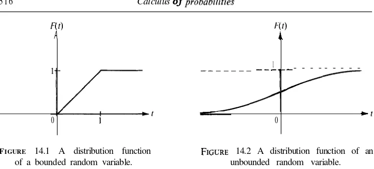
14. CALCULUS OF PROBABILITIES

(18)

14.10 Uniform distribution over an interval

14.17 Distributions of functions of random variables 14.18 Exercises

14.19 Distributions of two-dimensional random variables 14.20 Two-dimensional discrete distributions

14.21 Two-dimensional continuous distributions. Density functions 14.22 Exercises

14.23 Distributions of functions of two random variables 14.24 Exercises

14.25 Expectation and variance

14.26 Expectation of a function of a random variable 14.27 Exercises

14.28 Chebyshev’s inequality 14.29 Laws of large numbers

14.30 The central limit theorem of the calculus of probabilities 14.3 Exercises

Suggested References

15. INTRODUCTION TO NUMERICAL ANALYSIS

15.1 Historical introduction

15.2 Approximations by polynomials

15.3 Polynomial approximation and linear spaces 15.4 Fundamental problems in polynomial approximation

15.11 Equally spaced interpolation points. The forward difference operator 15.12 Factorial polynomials

15.13 Exercises

15.14 A minimum problem relative to the max norm

(19)

PART

(24)

(25)

1 LINEAR SPACES

1.1 Introduction

Throughout mathematics we encounter many examples of mathematical objects that can be added to each other and multiplied by real numbers. First of all, the real numbers themselves are such objects. Other examples are real-valued functions, the complex numbers, infinite series, vectors in n-space, and vector-valued functions. In this chapter we discuss a general mathematical concept, called a linear space, which includes all these examples and many others as special cases.

Briefly, a linear space is a set of elements of any kind on which certain operations (called

addition and multiplication by numbers) can be performed. In defining a linear space, we do not specify the nature of the elements nor do we tell how the operations are to be performed on them. Instead, we require that the operations have certain properties which we take as axioms for a linear space. We turn now to a detailed description of these axioms.

1.2 The definition of a linear space

Let denote a set of objects, called elements. The set is called a linear space if it satisfies the following ten axioms which we list in three groups.

Closure axioms

AXIOM C L O S U R E U N D E R A D D I T I O N. For every pair of elements x and y in V there

corresponds a unique element in V called the sum of x and y, denoted by x + y .

AXIOM 2. CLOSURE UNDER MULTIPLICATION BY REAL NUMBERS. For every x in V and

every real number a there corresponds an element in V called the product of a and x, denoted by ax.

Axioms for addition

AXIOM 3. COMMUTATIVE LAW. For all x and y in we have x + y = y + x.

(26)

AXIOM EXISTENCEOFZEROELEMENT. There is an element in denoted by 0, such that

V .

AXIOM 6. EXISTENCEOFNEGATIVES. For x in V, the element 1)x has the property 0 .

Axioms for multiplication by numbers

AXIOM 7. ASSOCIATIVE LAW. For every x in V and all real numbers a and b, we have a(bx) = (ab)x.

AXIOM 8. DISTRIBUTIVE LAW FOR ADDITION IN For all x andy in V and all real a,

we hare

+ y ) = ax + ay .

AXIOM 9. DISTRIBUTIVE LAW FOR ADDITION OF NUMBERS. For all in V and all real a and b, we

(a + b)x = ax + bx.

AXIOM EXISTENCE OF IDENTITY. For every in we have lx = x.

Linear spaces, as defined above, are sometimes called real linear spaces to emphasize the fact that we are multiplying the elements of V by real numbers. If real number is replaced by complex number in Axioms 2, 7, 8, and 9, the resulting structure is called a complex linear space. Sometimes a linear space is referred to as a linear vector space or simply a vector space; the numbers used as multipliers are also called scalars. A real linear space has real numbers as scalars; a complex linear space has complex numbers as scalars. Although we shall deal primarily with examples of real linear spaces, all the theorems are valid for complex linear spaces as well. When we use the term linear space without further designation, it is to be understood that the space can be real or complex.

1.3 Examples of linear spaces

If we specify the set V and tell how to add its elements and how to multiply them by numbers, we get a concrete example of a linear space. The reader can easily verify that each of the following examples satisfies all the axioms for a real linear space.

EXAMPLE 1. Let V R , the set of all real numbers, and let x + y and ax be ordinary

addition and multiplication of real numbers.

EXAMPLE 2. Let V the set of all complex numbers, define + y to be ordinary

(27)

Examples of linear spaces

by the real number a. Even though the elements of are complex numbers, this is a real linear space because the scalars are real.

EXAMPLE 3. Let = the vector space of all n-tuples of real numbers, with addition

and multiplication by scalars defined in the usual way in terms of components.

EXAMPLE 4. Let be the set of all vectors in orthogonal to a given vector

If = 2, this linear space is a line through 0 with as a normal vector. If = 3, it is a plane through 0 with as normal vector.

The following examples are called function spaces. The elements of V are real-valued functions, with addition of two functions f and defined in the usual way:

(f + g)(x) =f(x) +

for every real in the intersection of the domains off and Multiplication of a function

f by a real scalar a is defined as follows: af is that function whose value at each x in the domain off is af (x). The zero element is the function whose values are everywhere zero. The reader can easily verify that each of the following sets is a function space.

EXAMPLE 5. The set of all functions defined on a given interval.

EXAMPLE 6. The set of all polynomials.

EXAMPLE 7. The set of all polynomials of degree where is fixed. (Whenever we

consider this set it is understood that the zero polynomial is also included.) The set of polynomials of degree equal to is not a linear space because the closure axioms are not satisfied. For example, the sum of two polynomials of degree need not have degree

EXAMPLE 8. The set of all functions continuous on a given interval. If the interval is

[a, b], we denote this space by C(a, b).

EXAMPLE 9. The set of all functions differentiable at a given point.

EXAMPLE 10. The set of all functions integrable on a given interval.

EXAMPLE 11. The set of all functions defined at with f(1) = 0. The number 0 is

essential in this example. If we replace 0 by a number c, we violate the closure axioms.

E X A M P L E 12. The set of all solutions of a homogeneous linear differential equation

y” + + = 0, where a and b are given constants. Here again 0 is essential. The set of solutions of a nonhomogeneous differential equation does not satisfy the closure axioms.

(28)

diverse examples in this way we gain a deeper insight into each. Sometimes special knowl-edge of one particular example helps to anticipate or interpret results valid for other examples and reveals relationships which might otherwise escape notice.

1.4 Elementary consequences of the axioms

The following theorems are easily deduced from the axioms for a linear space.

TH EO REM U N IQ U EN ESS O F TH E Z ERO ELEM EN T. any linear space there is one and only one zero element.

Proof. Axiom 5 tells us that there is at least one zero element. Suppose there were two, say 0, and 0,. Taking x = and 0 = 0, in Axiom 5, we obtain + = Similarly, taking x = 02 and 0 = we find 02 + 0, = 02. But + 02 = 02 + 0, because of the commutative law, so 0, = 02.

THEOREM 1.2. UNIQUENESS OF NEGA TIVE ELEMENTS. In any linear space every element has exactly one negative. That is, for every x there is one and only one y such that x + y = 0.

Proof. Axiom 6 tells us that each x has at least one negative, namely (- 1)x. Suppose x has two negatives, say and Then x + = 0 and x + = 0. Adding to both members of the first equation and using Axioms 5, 4, and 3, we find that

and

+ + = + x) + = 0 +

Therefore = so x has exactly one negative, the element (- 1)x.

Notation. The negative of x is denoted by The difference y x is defined to be the sum y (-x) .

The next theorem describes a number of properties which govern elementary algebraic manipulations in a linear space.

THEOREM 1.3. In a given linear space, let x and y denote arbitrary elements and let a and b denote arbitrary scalars. Then w e‘have the follow ing properties:

(a) Ox = 0. ( b ) a 0 = 0 .

( c ) ( - a ) x = - ( a x ) = a ( - x ) .

( d ) I f a x = O , t h e n e i t h e r a = O o r x = O . ( e ) t h e n x = y . ( f )

+ = + =

(29)

Exercises 7

We shall prove (a), (b), and (c) and leave the proofs of the other properties as exercises.

Proof of (a). Let = Ox. We wish to prove that = 0. Adding z to itself and using

In Exercises 1 through 28, determine whether each of the given sets is a real linear space, if addition and multiplication by real scalars are defined in the usual way. For those that are not, tell which axioms fail to hold. The functions in Exercises 1 through 17 are real-valued. In Exer-cises 3, 4, and 5, each function has domain containing 0 and 1. In ExerExer-cises 7 through 12, each domain contains all real numbers.

6. All step functions defined on [0, 11. All increasing functions.

7. 12. All functions with period

13. All f integrable on [0, with f( x) dx = 0.

14. All f integrable on [0, with f( x) dx 0 .

15. All f = x) for all x.

16. All Taylor polynomials of degree for a fixed (including the zero polynomial). 17. All solutions of a linear second-order homogeneous differential equation’ y” + +

= 0, where P and Q are given functions, continuous everywhere. 18. All bounded real sequences. 20. All convergent real series.

19. All convergent real sequences. 21. All absolutely convergent real series. 22. All vectors (x, y, z) in with z = 0.

23. All vectors (x, y, z) in with x = 0 or y = 0. 24. All vectors (x, y, z) in with y = 5x.

25. All vectors (x, y, z) in with 3x + = 1, z = 0.

26. All vectors (x, y, z) in which are scalar multiples of 3).

27. vectors (x, y, z) in whose components satisfy a system of three linear equations of the form :

(30)

28. All vectors in that are linear combinations of two given vectors A and B.

29. Let V = the set of positive real numbers. Define the “sum” of two elements x and in V to be their product x (in the usual sense), and define “multiplication” of an element x in V by a scalar c to be Prove that V is a real linear space with 1 as the zero element. 30. (a) Prove that Axiom 10 can be deduced from the other axioms.

(b) Prove that Axiom 10 cannot be deduced from the other axioms if Axiom 6 is replaced by Axiom 6’: For every x in V there is an element in V such that x = 0.

3 1. Let be the set of all ordered pairs of real numbers. In each case determine whether or not is a linear space with the operations of addition and multiplication by scalars defined as indicated. If the set is not a linear space, indicate which axioms are violated.

+ = = 0).

+ = =

= + =

32. Prove parts (d) through (h) of Theorem 1.3.

1.6 Subspaces of a linear space

Given a linear space let S be a subset of If is also a linear space, with the same operations of addition and multiplication by scalars, then is called a

of The next theorem gives a simple criterion for determining whether or not a subset of a linear space is a subspace.

T H E O R E M 1.4. Let S be a subset of a linear space V. Then S is a

if and only if S satisfies the closure axioms.

Proof. If S is a subspace, it satisfies all the axioms for a linear space, and hence, in particular, it satisfies the closure axioms.

Now we show that if S satisfies the closure axioms it satisfies the others as well. The commutative and associative laws for addition (Axioms 3 and 4) and the axioms for multiplication by scalars (Axioms 7 through 10) are automatically satisfied in S because they hold for all elements of V. It remains to verify Axioms 5 and 6, the existence of a zero element in S, and the existence of a negative for each element in S.

(31)

Dependent and independent sets in a linear space 9

Different sets may span the same subspace. For example, the space is spanned by

each of the following sets of vectors: + The space

of all of degree is spanned by the set of + 1 polynomials . . .

It is also spanned by the set t/2, . . . , + and

by

+ + . . . , (1 + The space of all polynomials is spanned by the infinite set of polynomials

t,

. .

A number of questions arise naturally at this point. For example, which spaces can be spanned by a finite set of elements? If a space can be spanned by a finite set of elements, what is the smallest number of elements required? To discuss these and related questions, we introduce the concepts of dependence, independence, bases, and dimension. These ideas were encountered in Volume I in our study of the vector space . Now we extend them to general linear spaces.

1.7 Dependent and independent sets in a linear space

DEFINITION. A set of elements in a linear space V is called dependent there is set of distinct elements in say . . . , and a corresponding set of scalars . . . , not all zero, such that

An equation = 0 with not all = is said to be a nontrivial representation of 0. The set S is called independent is not dependent. In this case, for all choices of distinct elements . . . , in and scalars . . . ,

implies

Although dependence and independence are properties of sets of elements, we also apply these terms to the elements themselves. For example, the elements in an independent set are called independent elements.

If is a finite set, the foregoing definition agrees with that given in Volume I for the space However, the present definition is not restricted to finite sets.

EXAMPLE 1. If a subset T of a set is dependent, then itself is dependent. This is

logically equivalent to the statement that every subset of an independent set is independent.

EXPMPLE 2. If one element in is a scalar multiple of another, then is dependent.

EXAMPLE 3. If 0 then is dependent.

(32)

Many examples of dependent and independent sets of vectors in were discussed in Volume I. The following examples illustrate these concepts in function spaces. In each case the underlying linear space V is the set of all real-valued functions defined on the real line.

EXAMPLE 5. Let , , = for all real The Pythagorean

identity shows that + = 0, so the three functions are dependent.

EXAMPLE 6. Let = for k = 0, . . . , and real. The set = , . .

is independent. To prove this, it suffices to show that for each n the n + polynomials

are independent. A relation of the form = 0 means that

= 0

k=O

for all real When = this gives = 0 . Differentiating (1.1) and setting = we find that 0. Repeating the process, we find that each coefficient is zero.

EXAMPLE 7. If a,,...,a, are distinct real numbers, the exponential functions

= . . . , u,(x) =

are independent. We can prove this by induction on n. The result holds trivially when 1 . Therefore, assume it is true for n 1 exponential functions and consider scalars such that

= 0.

Let be the largest of the n numbers a,, . . . , a,. Multiplying both members of (1.2)

by we obtain

If k the number is negative. Therefore, when x + co in Equation each term with k tends to zero and we find that = 0. Deleting the Mth term from (1.2) and applying the induction hypothesis, we find that each of the remaining n 1 coefficients is zero.

THEOREM 1.5. = be an independent set consisting of k elements in a

linear space V and let L(S) be the spanned by Then every set of k + 1 elements in L(S) is dependent.

Proof. The proof is by induction on k, the number of elements in S. First suppose

(33)

Dependent and independent sets in a linear space 1 1 multiple of say = and = where and are not both 0. Multiplying

by and by and subtracting, we find that

= 0.

This is a nontrivial representation of 0 soy, and are dependent. This proves the theorem when k = 1 .

Now we assume the theorem is true for k 1 and prove that it is also true for k. Take any set of k + 1 elements in L(S), say T = , . . , . We wish to prove that Tis dependent. Since each is in L(S) we may write

k = a,

f o r e a c h i = , k + 1 . We examine all the scalars that multiply and split the proof into two cases according to whether all these scalars are 0 or not.

CASE 1. = 0 for every i = . . . , k + . In this case the sum in (1.4) does not involve so each in T is in the linear span of the set S’ = . . . , . But S’ is independent and consists of k 1 elements. By the induction hypothesis, the theorem is true for k 1 so the set T is dependent. This proves the theorem in Case 1.

CASE 2. Not all the are zero. Let us assume that a,, 0. (If necessary, we can renumber the y’s to achieve this.) Taking i = 1 in Equation (1.4) and multiplying both members by where we get

k

+ .

From this we subtract Equation (1.4) to get k

j

k + 1 . This equation expresses each of the k elements as a linear combination of the k 1 independent elements . . . , . By the induction hypothesis, the k elements must be dependent. Hence, for some choice of scalars . . . ,

not all zero, we have

from which we find

(34)

1.8 Bases and dimension

DEFINITION. A jinite set of elements in a linear space V is called basis V

S is independent and spans V. The space V is it has a jinite basis, or if V consists of 0 alone. Otherwise, V is called injinite-dimensional.

THEOREM 1.6. Let V be a linear space. Then every basis for V

has the same number of elements.

Proof. Let S and T be two finite bases for V. Suppose S consists of k elements and T

consists of m elements. Since S is independent and spans V, Theorem 1.5 tells us that every set of k + 1 elements in Vis dependent. Therefore, every set of more thank elements in V is dependent. Since T is an independent set, we must have m k. The same argu-ment with and T interchanged shows that k m . Therefore k = m .

DEFINITION. If a linear space V has a basis of n elements, the integer n is called the

dimension of V. We write = dim V.

If

V = we say V has dimension 0.

EXAMPLE 1. The space has dimension n. One basis is the set of unit coordinate

vectors.

EXAMPLE 2. The space of all polynomials p(t) of degree n has dimension n + 1 . One

basis is the set of + 1 polynomials . . . , Every polynomial of degree n is a linear combination of these n + 1 polynomials.

EXAMPLE 3. The space of solutions of the differential equation y” = 0 has

dimension 2. One basis consists of the two functions = = Every solution is a linear combination of these two.

E X A M P L E 4. The space of all polynomials p(t) is infinite-dimensional. Although the

infinite set . . spans this space, set of polynomials spans the space.

THEOREM 1.7. Let V be a jinite-dimensional linear space with dim V = n. Then we

have the following:

(a) Any set of independent elements in V is a of some basis for V.

(b) Any set of n independent elements is a V.

Proof. To prove (a), let = . . . , be any independent set of elements in V.

If L(S) = V, then is a basis. If not, then there is some element y in V which is not in

L(S). Adjoin this element to and consider the new set S’ = . . . , y} . If this set were dependent there would be scalars . . . , not all zero, such that

(35)

Exercises 13

is independent but contains k + 1 elements. If = then S’ is a basis and, since S is a subset of S’, part (a) is proved. If is not a basis, we can argue with S’ as we did with S, getting a new set which contains k 2 elements and is independent. If S” is a basis, then part (a) is proved. If not, we repeat the process. We must arrive at a basis in a finite number of steps, otherwise we would eventually obtain an independent set with

+ 1 elements, contradicting Theorem 1.5. Therefore part (a) is proved.

To prove (b), let S be any independent set consisting of elements. By part (a), S is a subset of some basis, say B. But by Theorem 1.6, the basis B has exactly elements, so

The coefficients in this equation determine an n-tuple of numbers (c,, . . . , that is uniquely determined by x. In fact, if we have another representation of as a linear combination of . . . , say = then by subtraction from we find that

= 0. B since the basis elements are independent, this implies t = The components of the ordered n-tuple (c,, . . . , determined by Equation (1.5) are called the components of x relative to the ordered basis (e, , . . . , e,).

Let denote the linear space of all real polynomials of degree where is fixed. In each of Exercises 11 through 20, let denote the set of all polynomials in satisfying the condition given. Determine whether or not is a of . If is a subspace, compute dim

21. In the linear space of all real polynomials describe the spanned by each of the following subsets of polynomials and determine the dimension of this subspace.

(36)

22. In this exercise, L(S) denotes the spanned by a subset of a linear space Prove each of the statements (a) through (f).

(a) L(S).

23. Let V be the linear space consisting of all real-valued functions defined on the real line.

Determine whether each of the following subsets of V is dependent or independent. Compute the dimension of the spanned by each set.

(f) {cos x, sin

In ordinary Euclidean geometry, those properties that rely on the possibility of measuring lengths of line segments and angles between lines are called metric properties. In our study of we defined lengths and angles in terms of the dot product. Now we wish to extend these ideas to more general linear spaces. We shall introduce first a generalization of the dot product, which we call an inner product, and then define length and angle in terms of the inner product.

The dot product x of two vectors x = . . . , x,) and = . . . , in was defined in Volume I by the formula

y =

In a general linear space, we write (x, instead of x for inner products, and we define the product axiomatically rather than by a specific formula. That is, we state a number of properties we wish inner products to satisfy and we regard these properties as axioms.

DEFINITION. A real linear space V is said to have an inner product for each pair of elements x and y in V there corresponds a unique real number (x, y) satisfying the following axioms for all choices of x, y, z in V and all real scalars c.

= (commutativity, or symmetry).

+ = + (distributivity, or linearity). (3) = (associativity, or homogeneity).

(37)

Inner products, Euclidean spaces. Norms 1 5 A real linear space with an inner product is called a real Euclidean space.

Note: Taking c = 0 in we find that = 0 for all

In a complex linear space, an inner product (x, is a complex number satisfying the same axioms as those for a real inner product, except that the symmetry axiom is replaced by the relation

sy mmetry )

where x) denotes the complex conjugate of (y, x). In the homogeneity axiom, the scalar multiplier c can be any complex number. From the homogeneity axiom and we get the companion relation

_ _

(3’) = (cy, x) = x) = y).

A complex linear space with an inner product is called a complex Euclidean ‘space. (Sometimes the term unitary space is also used.) One example is complex vector space

discussed briefly in Section 12.16 of Volume I.

Although we are interested primarily in examples of real Euclidean spaces, the theorems of this chapter are valid for complex Euclidean spaces as well. When we use the term Euclidean space without further designation, it is to be understood that the space can be real or complex.

The reader should verify that each of the following satisfies all the axioms for an inner product.

EXAMPLE 1. In let y) = . , the usual dot product of and y.

EXAMPLE 2. If x = and y = , are any two vectors in define (x, y) by

the formula

= + +

This example shows that there may be more than one inner product in a given linear space.

EXAMPLE 3. Let denote the linear space of all real-valued functions continuous

on an interval [a, b]. Define an inner product of two functions and by the formula

=

.

This formula is analogous to Equation (1.6) which defines the dot product of two vectors i n The function values and play the role of the components and , and integration takes the place of summation.

(38)

EXAMPLE 4. In the space b), define

where w is a fixed positive function in b). The function w is called a weightfunction.

In Example 3 we have w(t) = 1 for all

EXAMPLE 5. In the linear space of all real polynomials, define

Because of the exponential factor, this improper integral converges for every choice of polynomials

THEOREM 1.8. a Euclidean space every inner product satisfies the Cauchy-Schwarz

inequality:

(x, for all andy in V.

Moreover, the equality sign holds only if x and y are dependent.

Proof. If either x = 0 or y = 0 the result holds trivially, so we can assume that both x and y are Let z = ax + by, where a and b are scalars to be specified later. We have the inequality (z, z) 0 for all a and b. When we express this inequality in terms of x and y with an appropriate choice of a and b we will obtain the Cauchy-Schwarz inequality.

To express z) in terms of x and y we use properties (2) and (3’) to obtain

by,

+

by)

= (ax, + (ax, by) + (by, ax) + (by, by)

= + + + 0.

Taking a = (y, y) and cancelling the positive factor y) in the inequality we obtain

+

we take b = . Then 6 = (y, x) and the last inequality simplifies to =

This proves the Cauchy-Schwarz inequality. The equality sign holds throughout the proof if and only if = 0. This holds, in turn, if and only if x and y are dependent.

EXAMPLE. Applying Theorem 1.8 to the space b) with the inner product =

dt , we find that the Cauchy-Schwarz inequality becomes

(39)

Inner products, Euclidean spaces. Norms 17 The inner product can be used to introduce the metric concept of length in any Euclidean space.

DEFINITION. In a Euclidean space the nonnegative number by the equation

is called the norm of the element x.

When the Cauchy-Schwarz inequality is expressed in terms of norms, it becomes

Since it may be possible to define an inner product in many different ways, the norm of an element will depend on the choice of inner product. This lack of uniqueness is to be expected. It is analogous to the fact that we can assign different numbers to measure the length of a given line segment, depending on the choice of scale or unit of measurement. The next theorem gives fundamental properties of norms that do not depend on the choice of inner product.

THEOREM 1.9. In a Euclidean space, every norm has the following properties for all elements x and y and all scalars c:

=

(positivity).

=

(homogeneity).

+ (triangle inequality).

The equality sign holds in (d) x = = or if y = cxfor some c > 0.

Proof. Properties (a), (b) and (c) follow at once from the axioms for an inner product. To prove (d), we note that

= + + +

The sum (x, y) + (x, y) is real. The Cauchy-Schwarz inequality shows that llyll ,

+ + + =

This proves (d). When y = cx , where c > 0, we have

(40)

DEFINITION. In a real Euclidean space the angle between two elements x and y is to be that number in the interval 0 w hich satisfies the equation

c os e =

Note: The inequality shows that the quotient on the right of (1.7) lies in the interval [ , so there is exactly one in [0, whose cosine is equal to this quotient.

1.12 Orthogonality in a Euclidean space

DEFINITION. In a Euclidean space tw o elements x and y are called orthogonal their

inner product is zero. A subset of V is an orthogonal set (x, y ) = 0 for every pair

of distinct elements x and y in S. An orthogonal set is called orthonormal each of its elements has norm 1.

The zero element is orthogonal to every element of V; it is the only element orthogonal to itself. The next theorem shows a relation between orthogonality and independence.

THEOREM 1.10. a Euclidean space every orthogonal set of elements is

independent. In particular, in a jinite- dimensional Euclidean space w ith dim V = every orthogonal set consisting of n elements is a basis for V.

Proof. Let S be an orthogonal set of elements in V, and suppose some finite linear combination of elements of is zero, say

where each S. Taking the inner product of each member with and using the fact that (xi , = 0 if i 1 , we find that = But 0 since 0 so = 0. Repeating the argument with replaced by we find that each = 0. This proves that is independent. If dim V = n and if consists of n elements, Theorem 1.7(b) shows that is a basis for V.

EXAMPLE. In the real linear space with the inner product =

let be the set of trigonometric functions . . given by

= cos nx, = sin nx, f o r n = If m n, we have the orthogonality relations

(41)

Orthogonality in a Euclidean space 1 9 so S is an orthogonal set. Since no member of S is the zero element, S is independent. The norm of each element of is easily calculated. We have = dx = and, for

n we have

nx dx =

Therefore, = and = for n 1 . Dividing each by its norm, we obtain an orthonormal set , . . where = Thus, we have

= = f o r

In Section 1.14 we shall prove that every finite-dimensional Euclidean space has an orthogonal basis. The next theorem shows how to compute the components of an element relative to such a basis.

THEOREM I 1. Let V he a Euclidean space dimension and

that = . . . , an orthogonal

[fan

element x is expressed as linear combination of the basis elements, say

= ,

its components relative to the ordered basis (e, , . . . , are given by

‘1.9)

particular, if is an orthonormal basis, each is given by

= (x, .

Proof. Taking the inner product of each member of (1.8) with we obtain

= =

= 0 if i This implies and when = we obtain (1.10). If . . . , e,} is an orthonormal basis, Equation (1.9) can be written in the form

1.11) (x, .

(42)

THEOREM 1.12. Let V be Euclidean space of dimension n, and assume

fhat {e,, . . . , e,} is an orthonormal basis for V. Then for every puir of elements x and y in V, we have

(1.12) (Parseval’s formula).

In particular, when x = y , we have

Proof, Taking the inner product of both members of Equation (1.11) withy and using the linearity property of the inner product, we obtain (1.12). When x = Equation (1.12) reduces to (1.13).

Note: Equation (1.12) is named in honor of A. (circa who obtained this type of formula in a special function space. Equation (1.13) is a generalization of the theorem of Pythagoras.

1.13 Exercises

1. Let x = . . . , x,) andy = . . . , be arbitrary vectors in . In each case, determine whether (x, y) is an inner product for if (x, y) is defined by the formula given. In case (x, y) is not an inner product, tell which axioms are not satisfied.

2. Suppose we retain the first three axioms for a real inner product (symmetry, linearity, and homogeneity but replace the fourth axiom by a new axiom (4’): (x, x) = 0 if and only if x = 0. Prove that either (x, x) > 0 for all x 0 or else (x, x) < 0 for all x 0.

[Hint: Assume (x, x) > 0 for some x 0 and y) < 0 for some 0. In the space spanned by {x, y), find an element 0 with (z, z) =

Prove that each of the statements in Exercises 3 through 7 is valid for all elements x and y in a real Euclidean space.

3. (x, y) = 0 if and only if + = . 4. (x, y) = 0 if and only if = +

5. (x, = 0 if and only if + for all real c. 6. (x y, x y) = 0 if and only if =

7. If x and y are elements making an angle with each other, then

(43)

Exercises

8. In the real linear space C(l, e), define an inner product by the equation

2 1

(a) = compute

(b) Find a linear polynomial g(x) = a + that is orthogonal to the constant function f(x) = 1.

9. In the real linear space C( let = dt . Consider the three functions given by

= , = = 1 +

Prove that two of them are orthogonal, two make an angle with each other, and two make an angle with each other.

10. In the linear space of all real polynomials of degree define

(a) Prove that is an inner product for .

(b) Compute = and

(c) = , find all linear polynomials orthogonal

In the linear space of all real polynomials, define dt .

(a) Prove that this improper integral converges absolutely for all polynomials and g.

(c) Compute when = = + 1 .

(d) Find all linear = a + orthogonal 1 +

12. In the linear space of all real polynomials, determine whether or not is an inner product if is defined by the formula given. In case is not an inner product, indicate which axioms are violated. In (c), and denote derivatives.

=

13. Let of all infinite sequences {x,} of real numbers for which the series converges. If x = and = are two elements of define

(a) Prove that this series converges absolutely.

Use the inequality to estimate the sum (b) Prove that is a linear space with (x, as an inner product. (c) Compute (x, if = = + 1) for 1.

(d) Compute (x, if = 1.

Let be the set of all real functions continuous on [0, + and such that the integral

(44)

(a) Prove that the integral for converges absolutely for each pair of functions f and in V.

[Hint: Use the inequality to estimate the integral f

(b) Prove that V is a linear space with (f, as an inner product.

(c) Compute = = where = 0, . . . .

15. In a complex Euclidean space, prove that the inner product has the following properties for all elements and z, and all complex a and

= (b) (x, + = +

16. Prove that the following identities are valid in every Euclidean space.

(a) = + + +

+ =

+

=

+

17. Prove that the space of all complex-valued functions continuous on an interval [a, b] becomes a unitary space if we define an inner product by the formula

=

where w is a fixed positive function, continuous on [a, b].

1.14 Construction of orthogonal sets. The Gram-Scltmidt process

Every finite-dimensional linear space has a finite basis. If the space is Euclidean, we can always construct an orthogonal basis. This result will be deduced as a consequence of a general theorem whose proof shows how to construct orthogonal sets in any Euclidean space, finite or infinite dimensional. The construction is called the Gram-Schmidt onalizationprocess, in honor of J. P. Gram (1850-1916) and E. Schmidt (18451921).

T H E O R E M 1.13. O R T H O G O N A L I Z A T I O N T H E O R E M. Let be ajinite o r

sequence of elements in a Euclidean space V, and let . . . , denote the

spanned by k of these elements. Then there is a corresponding sequence of elements in V which has the following properties for each integer k:

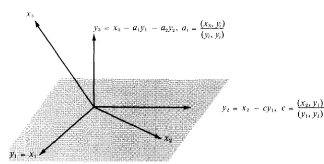
Proof. We construct the elements . . . , by induction. To start the process, we take = Now assume we have constructed . . . , so that (a) and (b) are satisfied when k = r . Then we define by the equation

(45)

Construction of orthogonal sets. The Gram- Schmidt process 2 3 where the scalars a,, . . . , a, are to be determined. For j the inner product of with is given by

since = if

. If

we can make orthogonal to by taking

(1.15) ₃

If then is orthogonal to for any choice of and in this case we choose Thus, the element is well defined and is orthogonal to each of the earlier elements , . . . , . Therefore, it is orthogonal to every element in the

This proves (a) when = r + 1.

To prove (b) when k = r + we must show that . . . , , . . . , given that . . . , = . . . , . The first r elements . . . , are in

and hence they are in the larger , . . . , The new element given by (1.14) is a difference of two elements in . . , so it, too, is in . . . , This proves that

Equation (1.14) shows that is the sum of two elements in , . . . , so a similar argument gives the inclusion in the other direction:

This proves (b) when k = r + 1. Therefore both (a) and (b) are proved by induction on k. Finally we prove (c) by induction on k. The case k = 1 is trivial. Therefore, assume (c) is true for k = r and consider the element . Because of (b), this element is in

so we can write

= +

where . .. , . We wish to prove that = 0. By property (a), both and are orthogonal to . Therefore, their difference, is orthogonal to . In other words, is orthogonal to itself, so = 0. This completes the proof of the

(46)

In the foregoing construction, suppose we have 0 for some Then (1.14) shows that is a linear combination of . . . and hence of . . . , so the elements . . . , are dependent. In other words, if the first k elements . . , are independent, then the corresponding elements , . . . , are In this case the coefficients in (1.14) are given by and the formulas defining , . . . , become

(1.16) = = for = . . . , k 1.

These formulas describe the Gram-Schmidt process for constructing an orthogonal set of elements . . . , which spans the same as a given independent set . . In particular, if . . . , is a basis for a finite-dimensional Euclidean space, . . . is an orthogonal basis for the same space. We can also convert this to an orthonormal basis by normalizing each element that is, by dividing it by its norm. Therefore, as a corollary of Theorem 1.13 we have the following.

THEOREM 1.14. Euclidean space has an orthonormal basis. If and y are elements in a Euclidean space, withy the element

is called the projection of x along y. In the Gram-Schmidt process we construct the element by subtracting from the projection of along each of the earlier elements . . . , Figure 1.1 illustrates the construction geometrically in the vector space

(47)

Construction of orthogonal sets. The Gram-Schmidt process 25

E X A M P L E 1. In find an orthonormal basis for the spanned by the three

vectors = (1, -1, 1, = (5, 1, 1, and (-3, -3, 1, -3).

Solution. Applying the Gram-Schmidt process, we find

= = (1, -1, 1,

= = =

= Yl + =

Since the three vectors must be dependent. But since and are

the vectors and are independent. Therefore is a of

dimension 2. The set is an orthogonal basis for this subspace. Dividing each of and by its norm we get an orthonormal basis consisting of the two vectors

EXAMPLE 2. The Legendre polynomials. In the linear space of all polynomials, with the

inner product (x, y) = dt , consider the infinite sequence , ,where

= When the orthogonalization theorem is applied to this sequence it yields another sequence of polynomials . . . , first encountered by the French mathe-matician A. M. Legendre (1752-1833) in his work on potential theory. The first few polynomials are easily calculated by the Gram-Schmidt process. First of all, we have

= 1 . Since

and = =

we find that

= = = t.

0

Next, we use the relations

to obtain

= =

0 1

Similarly, we find that

(48)

We shall encounter these polynomials again in Chapter 6 in our further study of differential equations, and we shall prove that

n!

1)“.

The polynomials given by

=

are known as the Legendrepolynomials. The polynomials in the corresponding orthonormal

are called the normalized Legendre

poly-nomials. From the formulas for . . . , given above, we find that

= = t = 1)) =

= + = +

1.15. Orthogonal complements. Projections

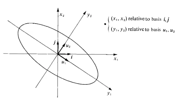
Let be a Euclidean space and let S be a finite-dimensional subspace. We wish to consider the following type of approximation problem: Given an element x in V, to deter-mine an element in S whose distance from x is as small as possible. The distance between two elements x and y is defined to be the norm .

Before discussing this problem in its general form, we consider a special case, illustrated in Figure 1.2. Here V is the vector space and S is a two-dimensional subspace, a plane through the origin. Given x in V, the problem is to find, in the plane S, that point nearest to x.

If x then clearly = x is the solution. If x is not in S, then the nearest point is obtained by dropping a perpendicular from x to the plane. This simple example suggests an approach to the general approximation problem and motivates the discussion that follows.

DEFINITION. Let S be a subset of a Euclidean space V. An element in V is said to be orthogonal to S if it is orthogonal to every element of S. The set of’ all elements orthogonal to S is denoted by and is called perpendicular.”

It is a simple exercise to verify that is a of V, whether or not S itself is one. In case S is a subspace, then is called the orthogonal complement of S.

(49)

Orthogonal complements. Projections 2 7

FIGURE 1.2 Geometric interpretation of the orthogonal decomposition theorem in

T H E O R E M 1.15. O R T H O G O N A L D E C O M P O S I T I O N T H E O R E M. Let V be a Euclidean space

and let S be of V. Then every element x in V can be represented uniquely as a sum of two elements, one in S and one in That is, we have

(1.17) where S and

Moreover, the norm of x is given by the Pythagorean formula

(1.18)

=

+

Proof. First we prove that an orthogonal decomposition (1.17) actually exists. Since S is finite-dimensional, it has a finite orthonormal basis, say {e, , . . . , e,}. Given define the elements and as follows:

(1.19) = (x, = x - s .

Note that each term (x, is the projection of x along . The element is the sum of the projections of x along each basis element. Since is a linear combination of the basis elements, lies in S. The definition of shows that Equation (1.17) holds. To prove that

lies in we consider the inner product of and any basis element . We have

= (x, e,) (s, .

But from we find that (s, = (x, e,), so is orthogonal to Therefore is orthogonal to every element in S, which means that .

Next we prove that the orthogonal decomposition (1.17) is unique. Suppose that x has two such representations, say

(50)

where and t are in and and are in We wish to prove that = t and = .

From we have t = so we need only prove that = 0. But

t Sand so t is both orthogonal to and equal to . Since the zero element is the only element orthogonal to itself, we must have t = 0. This shows that the decomposition is unique.

Finally, we prove that the norm of is given by the Pythagorean formula. We have

the remaining terms being zero since and are orthogonal. This proves (1.18).

DEFINITION. Let be a of a Euclidean space and let

. . . , e,} be an orthonormal basis for S.

If

x V, the element by the equation

= (x,

is called the projection of x on the S.

We prove next that the projection of x on is the solution to the approximation problem stated at the beginning of this section.

1.16 Best approximation of elements a Euclidean space by elements in a dimensional

T H EO REM 1.16. A PPRO X IM A T IO N T H EO REM . Let be a of

a Euclidean space V, and let x be any element o f V. Then the projection o f x on is nearer to x than any other element o f S. That is, is the projection o f x on we have

for all t in the equality sign holds if and only if t = s.

Proof. By Theorem 1.15 we can write x + where and Then, for any t in we have

x t = (x s) + (s t) .

Since and x = this is an orthogonal decomposition of x so its norm is given by the Pythagorean formula

=

+

But 0, so we have with equality holding if and only if

(51)

Best approximation of elements in a Euclidean space 29

EXAMPLE 1. Approximation of continuous functions on by trigonometric polynomials.

Let = the linear space of all real functions continuous on the interval and define an inner product by the equation g) = dx . In Section 1.12 we exhibited an orthonormal set of trigonometric functions . . . , where

=

= cos kx = f o r

The 2n + 1 elements . . , span a S of dimension 2n + 1. The ele-ments of are called trigonometric polynomials.

denote the projection off on the S. Then we have

(1.22) ₌

The numbers are called Fourier off. Using the formulas in we can rewrite (1.22) in the form

(1.23) where

f,(x) = cos +

= cos kx dx , = 1 f(x) sin kx dx

0

The approximation theorem tells us that the trigonometric poly-nomial in (1.23) approximates better than any other trigonometric polynomial in in the sense that the norm is as small as possible.

EXAMPLE 2. Approximation of continuous functions on by polynomials

of

degree n. Let = C(- the space of real continuous functions on [- 1, and let

= The + 1 normalized Legendre polynomials . . . ,

introduced in Section 1.14, span a S of dimension n + 1 consisting of all poly-nomials of degree n. let denote the projection off on S. Then we have

=

.

This is the polynomial of degree for which the norm is smallest. For example, = sin the coefficients are given by

=

sin dt.

(52)

Therefore the linear which is nearest to sin on [- is

Since = 0, this is also the nearest quadratic approximation.

1.17 Exercises

In each case, find an orthonormal basis for the of spanned by the given vectors.