The impact of climate change on the risk of forest
and grassland fires in Australia
A. J. Pitman&G. T. Narisma&J. McAneney
Received: 30 June 2005 / Accepted: 15 November 2006 / Published online: 17 March 2007
#Springer Science + Business Media B.V. 2007
Abstract We explore the impact of future climate change on the risk of forest and grassland fires over Australia in January using a high resolution regional climate model, driven at the boundaries by data from a transitory coupled climate model. Two future emission scenarios (relatively high and relatively low) are used for 2050 and 2100 and four realizations for each time period and each emission scenario are run. Results show a consistent increase in regional-scale fire risk over Australia driven principally by warming and reductions in relative humidity in all simulations, under all emission scenarios and at all time periods. We calculate the probability density function for the fire risk for a single point in New South Wales and show that the probability of extreme fire risk increases by around 25% compared to the present day in 2050 under both relatively low and relatively high emissions, and that this increases by a further 20% under the relatively low emission scenario by 2100. The increase in the probability of extreme fire risk increases dramatically under the high emission scenario by 2100. Our results are broadly in-line with earlier analyses despite our use of a significantly different methodology and we therefore conclude that the likelihood of a significant increase in fire risk over Australia resulting from climate change is very high. While there is already substantial investment in fire-related management in Australia, our results indicate that this investment is likely to have to increase to maintain the present fire-related losses in Australia.
DOI 10.1007/s10584-007-9243-6
A. J. Pitman (*)
Climate Change Research Centre, The University of New South Wales, Sydney, NSW 2052, Australia e-mail: [email protected]
G. T. Narisma
Center for Sustainability and the Global Environment, Nelson Institute for Env. Studies, University of Wisconsin, Madison, 1710 University Avenue, Madison, WI 53726, USA
J. McAneney
1 Introduction
There is a history of fire in Australia exceeding 400,000 years with high variability in fire frequency associated with natural climate variability (Kershaw et al. 2002). A substantial increase in fire frequency occurred about 38,000 years ago. This was probably related to human activity given that there is little evidence for a coincident change in climate. A second peak in fire occurrence was associated with European settlement in 1788 (Kershaw et al. 2002). Currently, around 5% of the Australian land surface is burned annually consuming approximately 10% of the net primary productivity of the continent (Pittock2003).
Fires in forests and grasslands cause substantial financial losses. About 200 homes were destroyed in the Sydney bush fires of 7–8th January 1994 (Gill and Moore1994; Ramsay et al. 1996) and 2,500 homes destroyed in the 16th February 1983 Ash Wednesday fires (Oliver et al.1984; Ramsay et al.1996) that also killed 75 people (Bureau of Meteorology1984). In other Australian fires, the 1974/75 bush fires in the Northern Territory burned 117 million hectares (Australian Bureau of Statistics1995) and more recently the 2003 Canberra bush fires destroyed 500 properties, killed four people and cost AUD$300 million (McLeod2003). On average, 84 homes are lost to bush fires each year (McAneney2005). McAneney (2005) also showed that there was about a 60% chance of residential home losses due to bush fire somewhere in Australia each year and that this situation has remained remarkably stable since the early twentieth Century. This consistency likely points to an element of climate control which in turn raises the question of how future changes in climate might affect fire risk.
There are many other costs associated with fire in Australia. Coronial inquiries are commonly established to investigate major fires. New South Wales, for example, has had at least seven bush fire inquiries since 1994 (Blong2004). Substantial investment in research has occurred (e.g. the Fire Code Reform Centre and the Bush Fire Cooperative Research Centre are multimillion dollar investments). There are major environmental costs associated with air pollution and impacts on human-health (Coghlan 2004) including during the fires (burns, smoke inhalation, Liu et al.1992) and post-fire psychological trauma (Sim2002). During the 2003 Canberra bush fire, the Mount Stromlo Observatory was destroyed. The Observatory, built in 1924, was of significant heritage value containing instruments that are irreplaceable. To deal with the financial costs of fire, considerable investment in fire services in Australia has occurred costing of order AUD$1,600 million in 2002–2003. A further investment, via the volunteer fire service has been estimated at AUD$460 million for Victoria (Hourigan2001) which approximates AUD$1,200 million Australia-wide. Due to the risks associated with fire, policy makers within Australia are interested in potential changes in fire regimes that might accompany greenhouse-related climate change (Beer and Williams1995).
Previous analyses of the impact of climate change on fire risk in Australia points to a likely increase. Beer and Williams (1995), Williams et al. (2001), Cary and Banks (1999) and Cary (2002) all found an increase in fire danger under increasing carbon dioxide (CO2)
Williams et al. (2001) also used the FDI and the CSIRO9 climate model (Watterson et al. 1995) coupled to a slab ocean model. A single 1×CO2and a single 2×CO2simulation were
performed at a horizontal resolution of 400×650 km. Daily data were used to calculate the FDI. The impact of increasing CO2included an increase in the number of days of very high
and extreme fire danger. When Williams et al. (2001) performed their analysis, the CSIRO9 model was state-of-the-art and it was then common to perform single scenarios for present and future climates. Further, they showed that the model performed reasonably over Australia in an evaluation of the current climate simulation. However, as computing resources have increased, the use of single scenarios for 1×CO2 and 2×CO2 and the
relatively coarse resolution of the climate model used are now recognised as limiting. Cary (2002) reviewed the evidence of the role of changing climate on fire regimes in Australia. He noted the limitations of scenarios developed by CSIRO (1996) in that they did not include projections of relative humidity or wind speeds (because they were not developed for the purposes of bush fire risk projection). Relative humidity and wind speed are required inputs to the McArthur bush fire danger index (McArthur 1967). Cary (2002) also noted strong regional variability in scenarios across the Australian continent. The lack of relative humidity data in the CSIRO (1996) scenarios forced Cary and Banks (1999) to assume that this variable would not change in the future, although Cary (2002) did account for changes in relative humidity in later work. Cary (2002) also performed the first simulations of bush fire change over Australia using a regional model embedded in a climate model.
Since the work by Beer and Williams (1995) and Williams et al. (2001), significant enhancements in climate modelling have occurred that allow the assumptions forced upon Cary and Banks (1999), for example, to be addressed. In this paper, we explore the impact of increasing CO2(and the subsequent changes in climate) on forest and grassland fire risk.
We attempt to address two major limitations in earlier studies: spatial resolution and use of single estimates of the future climate (although note that the CSIRO1996 scenarios were based on multiple climate models). To address the coarse resolution of previous estimates we use a regional climate model driven at the boundaries by the CSIRO climate model (see Section2.1). To address limitations that result from single projections of the future we use two scenarios that reflect relatively low and relatively high emissions (see Section2.1). We then perform four realizations for each of the present day (the control), 2050 and 2100 for each emission scenario and assess the change in fire risk using the FDI and a grassland fire danger index (GDI) in terms of the percentage change in the mean value and the change in the probability density function of the index. The use of multiple realizations, at least with the global and regional climate models, helps address areas of uncertainty in any projection sourced from an under-sampling of climate forcing. It also allows a sample of sufficient size to explore probabilities of change as distinct from the commoner assessment of a percentage change. Despite these attempts to reduce some aspects of uncertainty, we agree with Cary (2002) that climate models remain tools with considerable uncertainties and for this reason this paper should be considered very much in the context of scenario development and not in the sense of climate prediction.
2 Methodology
2.1 Regional climate model configuration
atmospheric modelling system (RAMS; Pielke et al. 1992; Liston and Pielke 2001) developed by the Colorado State University coupled to the General Energy and Mass Transport Model (GEMTM; Chen and Coughenor1994; Eastman et al.2001). RAMS is a flexible modelling system that has been extensively used to study weather and climate (see Pielke et al. 1998). RAMS has been shown to simulate the Australian January rainfall amounts and temperatures well (Peel et al.2005) and has proved useful for exploring the impacts of land cover change over Australia (Narisma and Pitman 2003). All RAMS simulations used in this paper used the Kain and Fritsch (1993) convection scheme and the Chen and Cotton (1987) shortwave and longwave radiation schemes. To provide the geographic distribution of vegetation over Australia, the classification from the Australian Surveying and Land Information Group (AUSLIG) was used. The 21 taxonomic groups provided by AUSLIG (1990) were mapped to the most structurally similar LEAF-2 plant functional type (see Peel et al. 2005). The details of our results would be sensitive to choices of individual parameterizations included in RAMS and thus it should not be inferred that our results are conclusive.
Regional climate models need to be initialized and provided with boundary conditions at the edge of the model’s domain. In this paper, RAMS was initialized and driven by boundary conditions taken from a transitory simulation of the CSIRO Mark 2 atmosphere-ocean model (Watterson and Dix 2003). The CSIRO model has a spatial resolution of approximately 3.2° latitude and 5.6° longitude and includes nine vertical layers for the atmosphere. The CSIRO model was used with two scenarios from the Special Report on Emissions Scenarios (SRES, Nakicenovic et al. 2000) that provide emission scenarios to 2100. We were provided with simulations that used B2 (low-moderate) emissions and A2 (high, particularly post 2050) emissions that project CO2levels of 456 and 532 ppmv by
2050 (B2, A2 scenarios, respectively), and 621 and 856 ppmv by 2100 (B2, A2 scenarios, respectively, see Table1). We used four Januaries near 2050 and four Januaries near 2100 to provide lateral boundary conditions to RAMS. The lateral boundary conditions were imposed on RAMS geographically remote from the continental surface. We also used four Januaries near 2000 as the control (by“near”we mean within ±2 years).
We therefore ran four January realizations for each emission scenario, for each time period. This is important since single realizations of a particular climate state can be misleading and while four realizations would not fully sample the statistics of the climate for a specific time period, they must sample more climate variability than a single realization. The number of realizations required to sample a given percentage of model variability has rarely been assessed. Wehner (2000) provides a guide to the number of realizations required to sample model variability but their results are from a global climate model while we have used a regional climate model. We used four realizations because this is better than one and more than four was prohibitively expensive in computational
Table 1 Statistics relating to the average of the four realizations for each experiment
Experiment CO2(ppmv) mean of FDI variance in FDI 5th percentile 95th percentile
Control 368 5.22 8.46 2.05 10.94
2050–A2 532 6.63 13.88 2.68 14.06
2050–B2 456 6.65 13.55 2.68 13.95
2100–A2 856 14.02 42.77 3.50 23.89
2100–B2 621 8.01 18.32 2.30 15.45
resources. Using RAMS, we performed simulations of the Australian January climate over an 80×100 domain at 56 km grid spacings. We simulated the January climate because this is a significant peak fire month in Australia. Lateral boundary conditions for RAMS were updated every 12-h which were found to be acceptable for simulations at a grid spacings of around 45 km by Denis et al. (2003) and were shown by Peel et al. (2005) to result in a good simulation of the current climate over Australia.
2.2 Fire indices
Where the AUSLIG (1990) data set identified land cover as woodland or forest we used the McArthur forest fire danger index (FDI, Noble et al. 1980) following Gill and Moore (1998) and Williams et al. (2001). This provides a measure of the fire risk which Williams et al. (2001) state is a valid indicator of forest fire danger at continental scales.
FDI¼2:0 exp½ 0:45þ0:987 logð ÞD 0:0345Hþ0:0338Tþ0:0234V ð1Þ
where H is the relative humidity (%),T is air temperature (°C),Vis wind velocity at a height of 10 m (m s−1) andDis a drought factor that we fixed in our experiments at the
maximum value (10.0). We calculated FDI every 4 h (this was the frequency at which model simulations could be saved given storage limitations) and summed these values over the month and then averaged over the total number of realizations. Since RAMS simulated H, T and V we did not need to derive these quantities post-simulation. Equation 1 is commonly used to indicate forest fire risk. Its value is that it compares the role of the principal climate variables that affect forest fire risk in the present climate. Due to the lack of any alternative strategy, we assume that the relationship between climate and forest fire risk expressed in Equation1will not change in the future.
Where the AUSLIG (1990) data set identified land cover as grassland or scrub we used the grassland fire danger index (GDI):
where C is a measure of curing which as per the drought index in Eq.1 we set to the maximum value of 10.0.
3 Results
3.1 Changes in forest and grassland fire potential, 2050
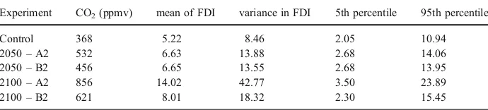
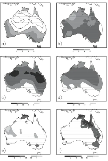
Figure1a and b show the simulated vales of FDI and GDI over Australia for the present day. The results for 2050 are shown in Fig.1c and d for the two emission scenarios (A2 and B2, respectively). The percentage change in FDI and GDI for 2050 is shown in Fig.1e and f. All panels show averages over four January realizations for each of 1×CO2and 2×CO2and
for ease of comparison between different panels, Fig.1a and b are identical. A higher value of FDI or GDI means that there is a greater likelihood of a fire starting and once ignited, there is a greater likelihood of the fire spreading, being more intense and more difficult to suppress (McArthur1967; Cary2002).
Figure1shows a typical climate projection where only CO2 and therefore climate are
changed. Under both emission scenarios, forest and grassland fire potential increases by 2050 by less than 10% over large areas (unshaded in Fig.1e, f). However, increases in FDI and GDI of 10–50% also occur over widespread areas. In comparison to Beer and Williams (1995), the apparent increase in fire potential appears high, but our simulations are limited to January (the peak bush fire month in much of New South Wales, NSW) while earlier work explored annual changes in potential.
As indicated above, both Fig. 1e and f show areas of higher increases. Under the A2 scenario, fire risk increases by more than 50% over some areas of Queensland (Fig.1e). In the B2 scenario the increases are largest over north west Australia (locally up to 200%). The areas where forest and grassland fire potential increase most in the A2 scenario are related to the projected changes in temperature in north west Australia where warming exceeds 3°C (Fig.2a) and to a decrease in relative humidity over Queensland (Fig.2c). A combination of these two changes explain the changes in fire risk in the B2 scenario (see Fig.2b and d). The role of changes in wind speed in affecting fire risk does not appear significant because the changes in wind speed in both the A2 and B2 scenarios is typically less than 1 km h−1
(Fig.2e and f). This supports Beer and Williams’(1995) result that changes in wind under increasing CO2 are likely to be less important than changes in temperature or relative
humidity although clearly in localized areas an increase in wind speed could be important. In our simulations wind speed decreased and hence tended to offset the increases in FDI and GDI that were driven by other aspects of climate. Lastly, our results demonstrate the limitations of Cary and Banks’(1999) use of a generalized climate change scenario that prevented them estimating a change in relative humidity.
Figure1f (relatively low B2 emission scenario) shows larger changes in FDI and GDI than Fig. 1e (relatively high A2 emission scenario) which might seem contradictory. By 2050 the A2 emission scenario prescribes a higher CO2 concentration (76 ppmv, see
Table 1) but the host climate model (like all climate models) is subject to internal variability. It happens that the CSIRO model simulates a greater change in 2050 in parts of Australia (but not globally) under the lower emission scenario. This is not critically important, rather it is an illustration of the dangers of using climate models without care and how multiple realizations of future projections are desirable.
Fig. 1 Actual FDI and GDI for the present day for theaA2 emission scenario andbB2 emission scenario. FDI and GDI for 2050 are shown in (c) and (d) respectively. Percent increase in FDI and GDI associated with CO2-induced climate change for 2050 are shown in (e) and (f). All results are averaged over four
Fig. 2 Impact on temperature (°C), relative humidity (%) and wind speed (m s−1) of increasing CO 2for
3.2 Changes in forest and grassland fire potential, 2100
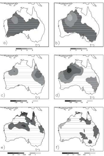
The potential increase in atmospheric CO2by 2100 is substantial (Table1) and this leads to
substantial climate changes in the CSIRO climate model that provides the lateral boundary conditions for the regional climate model simulations. The impact of these changes is shown in Fig.3. As with Fig.1, the current simulation of FDI and GDI is shown (Fig.3a for the A2 scenario and Fig.3b for the B2 scenario) to aid comparison with the projections for 2100 (Fig.3c and d).
In contrast to the 2050 projections where the results for emission scenarios A2 and B2 were generally similar in magnitude, at least over the eastern and southern states, the 2100 projections show marked differences. Under the A2 scenario, the increase in fire potential exceeds 50% compared to the current climate over most of the continent (Fig.3e). In the B2 scenario, fire potential increases by considerably less (generally 25–50%). In general, the increase in fire risk by 2100 under the B2 scenario is not much greater than by 2050. Comparing Figs.1f and3f suggests little increase in fire risk except along the Queensland coast and some areas of the sub-tropics. The potential for fire under the A2 scenario is very much higher by 2100 (Fig.3e) than in 2050 (Fig.1e) over much of the continent.
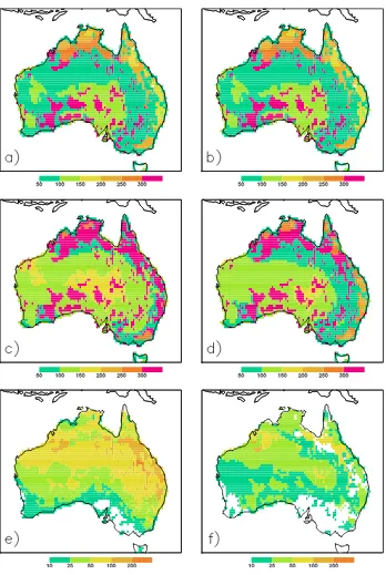
The pattern of changes in FDI and GDI mirror the simulated warming pattern and declines in relative humidity (Fig. 4). Figure 4a and b show widespread warming over Australia by 2100, commonly exceeding 5–6°C under the A2 scenario but rarely exceeding 3–4°C in the B2 scenario. Similarly, the relative humidity is reduced in the A2 scenario by more than 20% by 2100, in contrast to a reduction of 10–20% in the B2 scenario. The more intense warming and the stronger reduction in relative humidity in the A2 scenario compared to the B2 scenario largely explains the differences between Fig.3e and f. The changes in wind speed are again quite small (mainly less than 1 km h−1, Fig. 4e and f).
Where changes are larger, they are reductions in wind speeds and hence and do not contribute to the increases in FDI and GDI seen in Fig.3.
As with the changes in FDI and GDI for 2050, there are similarities between the A2 and B2 scenarios for the major urban centres. The projections agree for Perth (10–25% increase) and Melbourne (no change). However, the higher emission scenarios under A2, and the higher warming and stronger decreases in relative humidity has a major impact on FDI and GDI for Canberra, Sydney and Brisbane. Under B2, Canberra is projected to increase by 10–25% while Brisbane and Sydney are projected to increase by 25–50%. Under the A2 scenario these increase to at least 50–100% in Brisbane and Sydney.
3.3 Point-based impact of climate and land cover change on forest fire potential
Fig. 4 Impact on temperature (°C), relative humidity (%) and wind speed (m s−1) of increasing CO 2for
the same fire season zone experiences peak fire impact (in terms of area burned) in January (Conroy 1996). We specifically did not choose one of the major urban centres since we wanted the following analysis to be illustrative and not interpreted as a specific prediction. While the chosen grid point is typical of a larger area we cannot extrapolate these results reliably to other areas. We did not want to average over regions or large numbers of grid points, because in calculating probabilities we needed to keep the highest spatial and temporal resolution possible for analysis. It is prohibitive to repeat the following analysis for enough individual grid points to be able to generalize the results nationally.
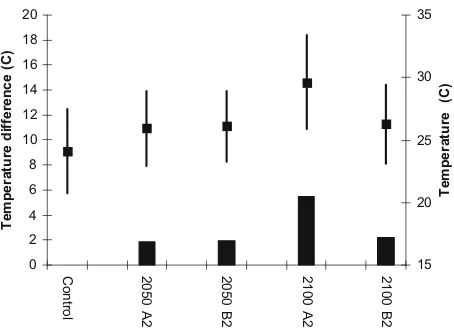
Figure 5 shows the simulated temperature and simulated temperature difference (experiment minus control for 2050 and 2100 for the A2 and B2 emission scenarios for this individual grid point (averaged over four realizations for each simulation). The stronger warming in the A2 emission scenario is particularly apparent. While the mean temperatures are noticeably higher in the A2 scenario the variability measured by the standard deviation is only marginally higher in the A2 (2100) simulations than in the other projections.
Figure6shows the equivalent point-based relative humidity. All four future projections
show reduced relative humidity of 10–15% for both B2 scenarios and the A2 scenario in
2050. Additional drying is apparent in the A2 scenario by 2100. Figure7shows the impact
0
Control 2050 A2 2050 B2 2100 A2 2100 B2
Temperature difference (C) 2050 and 2100 for the A2 and B2 emission scenarios. Thethick ver-tical barsshow the simulated temperature difference from the control (left hand axis). Thesmall squareshows the actual simulated mean and thethin barsshow ± one standard deviation from the mean (right hand axis). Units are °C and all results are averaged over six 4-hourly simulated temperatures over
Control 2050 A2 2050 B2 2100 A2 2100 B2
Relative humidity difference (%)
of the scenarios on wind speed with a generally reduced wind speed (at this single point) in the future but by quite small amounts. These changes are not sufficient to have a noticeable impact on the FDI.
Using 4-hourly temperature, relative humidity and windspeed data, we calculate the instantaneous FDI and then use the Bestfit software within a commercial Monte Carlo simulation package (@Risk, Palisade Corporation, NY, 2002) to fit probability density functions (PDF). The software fits data to distributions and ranks these according to goodness-of-fit statistics. Most appropriate distributions were determined either on the basis of the Anderson–Darling statistic, which places equal emphasis on the tails as well as the main body of the data (Vose1996), or by eye, taking into consideration realistic limits.
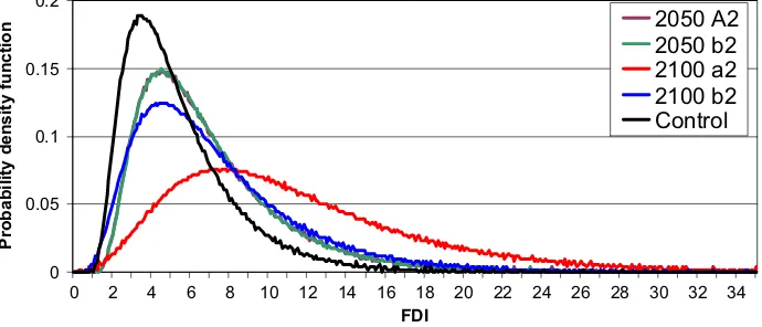
Figure8shows the results of this analysis. The data was well-represented by an Inverse Gaussian distribution (Vose 1996), its skewed shape expected given the non-linearity of Eq.1and the multi-variable dependence of the FDI. We note that our choice of distributions is purely descriptive and implies no mechanistic constraints over the data, a feature also true of Eq.1. Table1gives key moments controlling the shape of the PDF including its mean and variance, 5th and 95th percentile values. For the purposes of projecting a change in
0
Control 2050 A2 2050 B2 2100 A2 2100 B2
Wind speed difference (km/h)
scale of the left hand axis (the difference) is reversed in sign and that 10, 20% etc is a reduction (i.e. control-experiment)
forest fire risk, this latter value, which represents extreme values of the FDI associated with very high fire risk, is especially valuable.
The increase in forest and grassland fire risk by 2100 under the B2 scenario represents a further 20% increase in the mean FDI over the 2050 projection. The mean of the distribution increases from 5.2 (control) to 6.65 (2050) to 8.01 (2100) and there is a noticeable increase in the variance. However, as seen in Fig.8, the shape of the PDF for the B2 scenario is quite similar between 2050 and 2100 with only a small increase in the value of FDI that is exceeded 5% of the time (the increase is from 13.95 to 15.45, Table1). The shape of the PDF for 2100 in the A2 scenario is very different to all other simulations. The mean increases from 6.6 (2050) to 14.02 (2100) and the variance increases from 13.88 to 42.77. More significantly the FDI value that is exceeded 5% of the time increases from 14.06 to 23.89. Thus, the distribution is shifted towards much more extreme values and rather than the probability of FDI values exceeding 20 being negligible as in all other scenarios, the PDF projects non-negligible probabilities of FDI values exceeding 25. Clearly, under the A2 scenario, at this single location there is a substantially increased forest fire risk in 2100 compared with the B2 scenario. We note that the shapes and location of these four curves are common to each realization–that is all four realizations for 2100 A2 are substantially similar to each other, and substantially different to all other results.
4 Discussion and conclusions
This paper has shown that there is a strong likelihood that future climate change will increase the risk of forest and grassland fire in Australia. Our results therefore agree with earlier findings including those of Beer and Williams (1995), Cary and Banks (1999), Williams et al. (2001) and Cary (2002). This is worthy of note because the models used, the approaches and the methodologies differed amongst these groups. Rather than using global climate model outputs as input to the McArthur (1967) model (e.g. Beer and Williams 1995; Williams et al. 2001) or using prescribed climate change scenarios with simple estimates on climate change or a weather generator (e.g. Cary and Banks1999; Cary2002), we used results from multiple Januaries close to 2050 and 2100 from two contrasting emission scenarios (A2, B2) to drive a high resolution regional climate model (RAMS) through four independent realizations. Given that a series of different approaches give the same basic results, our confidence that increasing CO2 will increase forest and grassland
fire risk over Australia should be considered high.
Our results show a clear increase in forest and grassland fire risk in 2050 across much of continental Australia. The magnitude of the increase in risk is relatively independent of whether the relatively low or relatively high emission scenario is used by the global climate model. The increased risk of forest and grassland fire is geographically variable and on the large scale the pattern of increase in risk is dependent on whether the A2 or B2 scenario is used in the global climate model. Our results confirm earlier analyses (e.g. Beer and Williams 1995) that the changes in wind speeds are not significant in explaining the changes in forest and grassland fire risk, rather risk is dominated by changes in temperature and relative humidity. Indeed, in our simulations wind speed decreased, offsetting increases in fire risk caused by changes in other climate variables.
NSW coast and more than 100% along the Queensland coast. In all our simulations, for all emission scenarios and for both 2050 and 2100 the impact on fire risk over coastal Western Australia close to Perth is more limited (less than 25% increase) and we find no increase in risk over Melbourne. This is because coastal Victoria experiences warming, but relatively low warming coupled to small decreases in relative humidity. The increases in risk along the Queensland coast from Brisbane to the NSW boarder is worrisome since it is coincident with the region of strongest population growth in Australia (data on regional population growth is available at the Australian Bureau of Statistics: http://www.abs.gov.au/). This places a growing population at increased risk of fire.
When a single point was explored for a location in New South Wales, it was shown that the probability density function of the FDI was systematically shifted towards more extreme values of FDI as a result of higher emissions. The most significant difference was the impact of the A2 scenario on the FDI at 2100 where the probabilities of far higher values of the FDI was shown.
A reasonable conclusion from our work is that the use of a different methodology (regional climate models forced at the boundaries by a global climate model) gives results that are consistent for the impact of future climate change with earlier work. A benefit of our approach is the ability to perform multiple realizations rather less expensively than the cost of those realizations with the full global climate model. A second conclusion is that all our simulations suggest significantly higher risk of forest and grassland fires over Australia under both the A2 (high) and B2 (low) emission scenarios. The impact of a sustained emissions regime at the A2 levels leads to a very significantly enhanced risk of forest and grassland fires beyond 2050. Thus the risk is realized further into the future, but it is not reasonable to assume that it would take until 2100 for this to occur.
A change in the frequency or intensity of fire in Australia would likely have severe consequences increasing economic losses and the costs of fire management strategies. A change in the frequency or intensity of fire in Australia would also dramatically affect plant population dynamics and plant community composition (Gill1997) placing species near an extinction threshold at risk (Cary2002). Given that this paper demonstrates that the risk is substantially lower in a low emission future (B2, 2100) compared to a high emission future (A2, 2100), it provides a further reason to explore urgently strategies to develop along a low-emissions pathway.
Williams et al. (2001) noted that any interpretation of the impact of climate change on fire risk must include an understanding of the limitations of the scenarios by recognition of the assumptions that are built into the climate models. There are very many limitations to our work that should be emphasised. First, we used a single global climate model and a single regional climate model and we recognise that a different pattern of changes in FDI would likely have been obtained had we used other models. We doubt that a different conclusion (that is, strong evidence for a substantial increase in forest and grassland fire risk in the future) would have been reached in our study since global climate models are consistent in projecting large scale warming as a result of increasing CO2(Houghton et al.
produce a reduction in the impact of climate change unless precipitation changed in ways that reduced the drought and curing indices used in Eqs.1and2.
A further significant limitation is harder to resolve. Climate models simulate the large scale mean climate well (McAvaney et al. 2001), but bush fire frequency is strongly correlated with extreme weather. Little analysis has been conducted of the capacity of climate models to simulate extreme weather. Further, in building algorithms to manage boundary conditions for regional climate models, the focus of the evaluation of regional climate models has understandably on the means rather than extremes. Thus, in Table1the numeric values of the 95th percentiles are lower than those that typically drive high risk fire weather. This is in part related to the sampling from the climate model of large-scale forcing fields that are necessarily spatially and temporally smoothed, coupled with boundary condition algorithms that are evaluated on mean model skill rather than extremes. Further, climate models’s skill in simulating extremes at the 95th percentile level have not commonly been reported and it is very likely that they have less skill than in the mean. Clearly, in simulating important phenomenon like bush fire risk, the capacity of the models to simulate the extremes at the 95th percentile and above is a key aspect and warrants further analysis in the future.
While we agree with Williams et al. (2001) that a climatically driven FDI and GDI is a useful measure to address the impact of climate change on fire we have some concerns over the use of the McArthur (1967) index. The index does not take into account any possible changes in wind direction and the dynamic behaviour of fire in association with the location of the fire in respect to the landscape. We suspect that a new index based on a physically-based understanding of climate-fire behaviour would be useful, perhaps building on Cary (2002). Overall, the limitations in our methodology means that we believe that the details of our results should be considered as projections of possible futures and not necessarily the most in terms of fire risk. However, we do not believe that our conclusion that climate change will increase the risk of forest and grassland fires and that the higher the emissions, the higher the increase in the fire risk is substantially affected by these limitations.
Uncertainty will remain in projections of future climates for the foreseeable future. The climate modelling community is aware of these uncertainties and some innovative approaches to assessing their magnitude have recently been explored (Murphy et al. 2004; Stainforth et al.2005). We believe that recent developments in climate modelling allow a reappraisal of Cary’s (2002) statement that“the preferred method to incorporate climate change into landscape models is via a weather generator.”We suggest that the types of models developed by McCarthy and Cary (2002) can now directly use climate model results downscaled dynamically to high resolution provided multiple realizations of each climate change scenario are performed. This will permit probabilistic projections of changes in forest and grassland fire risk to be made that include uncertainties in the methodologies used to generate the results. We note here that our simulations were conducted at 56 km resolution but we have used a multiply-nested version of RAMS to a resolution of 1 km (Gero et al.2006). Thus the spatial resolution required for landscape scale fire projection is now possible from regional climate models.
In summary, we used two climate change projections as lateral boundary conditions to explore how forest and grassland fire risk might change over Australia for 2050 and 2100. We found, as have others before us, that there is a general increase in fire risk over Australia as the climate warms. This was common to both emission scenarios for both 2050 and 2100. However, the impact of the higher emissions in the A2 scenario led to a very much higher risk of forest and grassland fires by 2100 than the B2 scenario. At a single point this was illustrated via the probability density function of the FDI. This was gradually shifted towards higher values of FDI in both emission scenarios in 2050 and in the B2 scenario for 2100 but was dramatically shifted towards higher extremes in 2100 for the A2 emission scenario. We conclude from this, with the caveats discussed above in mind, that Australia will be significantly more exposed to forest and grassland fire risk in the future. A corollary to this is that lower emission scenarios will reduce this exposure and thereby substantially reduce costs associated with fire and fire prevention.
Acknowledgements We thank Roger A. Pielke Sr. for providing RAMS. Ian Watterson provided the CSIRO forcing data. G. T. Narisma was supported by a MUIPGRA scholarship. We also thank AC3 for providing supercomputing resources and Achim Casties for technical help. We thank three anonymous reviewers for their comments, advice and insight.
References
AUSLIG (1990) Vegetation: atlas of Australian resources, 3rd Series, vol. 6. Australian Surveying and Land Information Group, Depart. Administrative Services, Canberra, p 64
Australian Bureau of Statistics (1995) ABS year book Australia 1995, (1301.0). ABS, Canberra, Australia Beer T, Williams AA (1995) Estimating Australian forest fire danger under conditions of doubled carbon
dioxide concentration. Clim Change 29:169–188
Blong R (2004) Residential building damage and natural perils: Australian examples and issues. Build Res Inf 32(5):379–390
Bureau of Meteorology (1984) Report on the meteorological aspects of the Ash Wednesday fires –16 February 1983. Australian Government Public Service, Canberra, p 143
Cary GJ, Banks JCG (1999) Fire regime sensitivity to global climate change: an Australian perspective. In: Innes JL, Beniston M, Verstraete MM (eds) Biomass burning and its inter-relationship with the climate system. Kluwer, pp 233–246
Chen C, Cotton WR (1987) The physics of the marine strato-cumulus-capped mixed layer. J Atmos Sci 44:2951–2977
Chen D-X, Coughenor MB (1994) GEMTM: a general model for energy and mass transfer of land surfaces and its application at the FIFE sites. Agric For Meteorol 68:145–171
Clark JS (1990) Twentieth-century climate change, fire suppression, and forest production and decomposition in northwestern Minnesota. Can J For Res 20:219–232
Coghlan BJ (2004) The human health impact of the 2001–2002“Black Christmas”bushfires in New South Wales, Australia: an alternative multidisciplinary strategy. J. Rural and Remote Environmental Health 3:18–28 Conroy RJ (1996) To burn or not to burn? A description of the history, nature and management of bushfires
within Ku-Ring-Gai Chase national park. Proc Linn Soc NSW 116:79–95
CSIRO (1996) Climate change scenarios for the Australian region. CSIRO Division of Atmospheric Research, Melbourne, Australia
Denis B, Laprise R, Caya D (2003) Sensitivity of a regional climate model to the resolution of the lateral boundary conditions. Clim Dyn 20: doi:10.1007/s00382-002-0264-6
Eastman JL, Coughenor MB, Pielke RA Sr (2001) The regional effects of CO2 and landscape change using a coupled plant and meteorological model. Glob Chang Biol 7:797–815
Gaertner MA, Christensen OB, Prego JA, Polcher J, Gallardo C, Castro M (2001) The impact of deforestation on the hydrological cycle in the western Mediterranean: an ensemble study with two regional climate models. Clim Dyn 17:857–873
Gardner RH, Hargrove WW, Turner GM, Romme WH (1996) Climate change, disturbances and landscape dynamics. In: Walker B, Steffen W (eds) Global change and terrestrial ecosystems. Cambridge University Press, Cambridge, pp 149–172
Gero AF, Pitman AJ, Narisma GT, Jacobson C, Pielke RA (2006) The impact of land cover change on storms in the Sydney Basin, Australia. Glob Planet Change 54:57–78
Gill AM (1997) From “mosaic” burning to the understanding of the fire-dynamics of landscapes. In: McKaige BJ, Williams RJ, Waggitt WM (eds) Bush fires 97: proceedings of the Australasian bush fire conference, pp 89–94
Gill AM, Moore PHR (1994) Some ecological research perspectives on the disastrous Sydney fires of January 1994. Proc. Of the second International Conference on Forest Fire Research, volume 1, pp 63–72 Gill AM, Moore PHR (1998) Big versus small fires: the bush fires of greater Sydney, January 1994. In:
Moreno JM (ed) Large forest fires. Backhuys, Leiden, pp 49–68
Giorgi F, Shields-Brodeur C, Bates GT (1994) Regional climate change scenarios over the United States produced with a nested regional climate model. J Climate 7:375–399
Houghton JT, Ding Y, Griggs DJ, Noger M, van der Linden PJ, Dai X, Maskell K, Johnson CA (eds) (2001) Climate change, 2001, The scientific basis. Contribution of Working Group 1 to the third assessment report of the Intergovernmental Panel on Climate Change. Cambridge University Press, Cambridge, UK, p 881 Hourigan M (2001) The value of the volunteer contribution, Consultant’s report to the Victorian Country Fire Authority cited in the CFA submission to the Economic Development Committee of the Parliament of Victoria
Jones RG, Murphy JM, Noguer M (1995) Simulation of climate change over Europe using a nested regional-climate model: I assessment of control regional-climate, including sensitivity to location of lateral boundaries. Quart J Roy Meteorol Soc 121:1413–1449
Kain JS, Fritsch JM (1993) Convective parameterization for mesoscale models: The Kain–Fritsch scheme. The representation of cumulus convection in numerical models. Meteor Monogr 24:165–170 Kershaw AP, Clark JS, Gill AM, D’Costa DM (2002) A history of fire in Australia. In: Bradstock RA,
Williams JE, Gill MA (eds) Flammable Australia–The fire regimes and biodiversity of a continent. Cambridge University Press, pp 3–25
Leung LR, Ghan SJ (1999) Pacific Northwest climate sensitivity simulated by a regional climate model driven by a GCM. Part I: control simulation. J Climate 12:2010–2030
Liston GE, Pielke RA Sr (2001) A climate version of the regional atmospheric modeling system. Theor Appl Climatol 68:155–173
Liu D, Tager IB, Balmes JR, Harrison RJ (1992) The effect of smoke inhalation on lung function and airway responsiveness in wildland fire fighters. Am Rev Respir Dis 146:1469–1473
McAvaney BJ, Covey C, Joussaume S, Kattsov V, Kitoh A, Ogana W, Pitman AJ, Weaver A, Wood RA, Zhao Z-C (2001)Model Evaluation, In Chapter 8 of Climate Change, 2001, The Scientific Basis. Contribution of Working Group 1 to the third assessment report of the Intergovernmental Panel on Climate Change. In: Houghton JT, Ding Y, Griggs DJ, Noger M, van der Linden PJ, Dai X, Maskell K, Johnson CA (eds). Cambridge University Press, Cambridge, UK
McCarthy MA, Cary GJ (2002) Fire regimes in landscapes: models and realities. In: Bradstock RA, Williams JE, Gill MA (eds) Flammable Australia–The fire regimes and biodiversity of a continent. Cambridge University Press, pp 77–94
McGregor JL, Gordon HB, Watterson I, Dix MR, Rotstayn LD (1993) The CSIRO 9-level atmospheric general circulation model. CSIRO Division of Atmospheric Research, Technical paper 26, CSIRO, Australia, p 89
McLeod R (2003) The inquiry into the Operational Response to the January 2003 Bush fires,http://www. cmd.act.gov.au/mcleod_inquiry/report.htm
Murphy JM, Sexton DM, Barnett DN, Jones GS, Webb MJ, Collins M, Stainforth DA (2004) Quantification of modelling uncertainties in a large ensemble of climate change simulations. Nature 430:768–772 Nakicenovic N, Alcamo J, Davis G, de Vries B, Fenhann J, Gaffin S, Gregory K, Grübler A, Jung T-Y, Kram T,
La Rovere EL, Michaelis L, Mori S, Morita T, Pepper W, Pitcher H, Price L, Riahi K, Roehrl A, Rogner H-H, Sankovski A, Schlesinger M, Shukla P, Smith S, Swart R, van Rooijen S, Victor N, Dadi Z (2000) IPCC special report on emissions scenarios. Cambridge University Press, Cambridge, UK, p 599
Narisma GT, Pitman AJ (2003) The impact of 200 years of land cover change on the Australian near-surface climate. J Hydrometeorol 4:424–436
Narisma GT, Pitman AJ (2004) The effect of including biospheric feedbacks on the impact of land cover change over Australia. Earth Interact 8(5):1–28
Noble IR, Barry GAV, Gill AM (1980) McArthur’s fire-danger meters expressed as equations. Aust J Ecology 5:201–203
Oliver J, Britton NR, James MK (1984) The Ash Wednesday bush fires in Victoria: 16 February 1983, Disaster Invest. Rep. 7, Cent. for Disaster Stud., James Cook Univ., Townsville, Queensland, Australia Palisade Corporation (2002) Guide to Using @RISK, Version 4.5, Feb. 2002, Newfield, NY, USA Peel D, Pitman AJ, Hughes L, Narisma GT (2005) The impact of an explicit representation of Eucalyptus on
the simulation of the January climate of Australia. Environ Model Softw 20:595–612
Pielke RA, Cotton WR, Walko RL, Tremback CG, Lyons WA, Grasso LD, Nicholls ME, Moran MD, Wesley DA, Lee TJ, Copeland JH (1992) A comprehensive meteorological modeling system-RAMS. Meteorol Atmos Phys 49:69–91
Pielke RA Sr, Avissar R, Raupach M, Dolman AJ, Zeng X, Denning AS (1998) Interactions between the atmosphere and terrestrial ecosystems: Influence on weather and climate. Glob Chang Biol 4:461–475 Pitman AJ, Narisma GT, Pielke R, Holbrook NJ (2004) The impact of land cover change on the climate of
south west Western Australia. J Geophys Res 109:D18109 doi:10.1029/2003JD004347
Pittock B (ed) (2003) Climate change: an Australian guide to the science and potential impacts. Australian Greenhouse Gas Office, Commonwealth of Australia, p 239
Ramsay GC, McArthur NA, Dowling VP (1996) Building in a fire-prone environment: research on building survival in two major bush fires. Proc Linn Soc NSW 116:133–140
Sim M (2002) Bushfires: are we doing enough to reduce the human impact? Occ Env Med 59:215–216 Stainforth DA, Aina T, Christensen C, Collins M, Faull N, Frame DJ, Kettleborough JA, Knight S, Martin A,
Murphy JM, Piani C, Sexton D, Smith LA, Spicer RA, Thorpe AJ, Allen MR (2005) Uncertainty in predictions of the climate response to rising levels of greenhouse gases. Nature 433:403–406 Vose D (1996) Quantitative risk analysis: a guide to Monte Carlo simulation modelling. Wiley, Chichester,
p 328
Watterson I, Dix M (2003) Simulated changes due to global warming in daily precipitation means and extremes and their interpretation using the gamma distribution. J Geophys Res 108:4397 doi:10.1029/2002JD002928 Watterson IG, Dix MR, Gordon HB, McGregor JL (1995) The CSIRO 9-level atmospheric general circulation
model and its equilibrium present and doubled CO2 climates. Aust Meteorol Mag 44:111–125 Wehner MF (2000) A method to aid in the determination of the sampling size of AGCM ensemble
simulations. Clim Dyn 16:321–331
Whetton PH, Rayner PJ, Pittock AB, Haylock MR (1994) An assessment of possible climate change in the Australian region based on an intercomparison of general circulation modeling results. J Climate 7:441–463 Williams AA, Karoly DJ, Tapper N (2001) The sensitivity of Australian fire danger to climate change. Clim