ENHANCEMENT OF SNOW COVER CHANGE DETECTION WITH SPARSE
REPRESENTATION AND DICTIONARY LEARNING
Divyesh Varade*, Onkar Dikshit,
Department of Civil Engineering, IIT Kanpur, 208016, Kanpur, India (varadi, onkar)@iitk.ac.in Commission VIII, WG VIII/6
KEY WORDS: Snow Cover Change Detection, NDSI, Sparse Representation, K-SVD, k-means clustering.
ABSTRACT:
Sparse representation and decoding is often used for denoising images and compression of images with respect to inherent features. In this paper, we adopt a methodology incorporating sparse representation of a snow cover change map using the K-SVD trained dictionary and sparse decoding to enhance the change map. The pixels often falsely characterized as ‘changes’ are eliminated using this approach. The preliminary change map was generated using differenced NDSI or S3 maps in case of Resourcesat-2 and Landsat 8 OLI imagery respectively. These maps are extracted into patches for compressed sensing using Discrete Cosine Transform (DCT) to generate an initial dictionary which is trained by the K-SVD approach. The trained dictionary is used for sparse coding of the change map using the Orthogonal Matching Pursuit (OMP) algorithm. The reconstructed change map incorporates a greater degree of smoothing and represents the features (snow cover changes) with better accuracy. The enhanced change map is segmented using k-means to discriminate between the changed and non-changed pixels. The segmented enhanced change map is compared, firstly with the difference of Support Vector Machine (SVM) classified NDSI maps and secondly with a reference data generated as a mask by visual interpretation of the two input images. The methodology is evaluated using multi-spectral datasets from Resourcesat-2 and Landsat-8. The k-hat statistic is computed to determine the accuracy of the proposed approach.
1. INTRODUCTION
Snow cover monitoring is one of the crucial aspects of water supply management in Northern Himalayas, which implies extracting changes in the regional snow cover using remote sensing techniques regularly. The monitoring of snow cover is significant in various aspects from concluding the glacier masses, denomination of fresh water availability, climate change and towards understanding the glacier-river hydrological processes. To this aspect, understanding the seasonal variation of the snow cover also indicates patterns on the river dynamics. Satellite remote sensing, provides a key insight into all these applications. In several of these applications the basic work flow follows the identification of snow in the land cover and change detection of the existent snow cover. In literature, the Normalized Differenced Snow Cover index has been widely used for snow cover monitoring and development of snow cover maps (Negi et al., 2005), a concept derived from the reflectance pattern of snow in visible and infrared spectrum of light.
Besides monitoring snow change detection techniques are also applied in various other applications in remote sensing of natural resource and earth observation. The most basic form of unsupervised change detection technique is the simple image differencing (Singh, 1989). Various enhancements to the changes obtained by differencing are possible using image processing techniques (Radke et al., 2005). Besides these there are various other techniques for change detection with several reviews available in literature (Mas, 1999 and Lu et al., 2005). Fang et al., (2011), uses a sparse representation method for change detection. Sparse representation is often used for compressing images, and the same functionality is utilized in image de-noising. Change detection maps usually contain several small clusters of pixels for changes which would usually be invalid & apparent due to
* Corresponding author. D. Varade, E-mail: [email protected], Tel: +91-512-259-6147
various reasons. Thus, sparse representation and decoding can be effectively applied to the elimination of these clusters. Celik (2009), introduces an unsupervised approach for change detection by separating the differenced image into a feature vector space generated from the eigen images, followed by k-means clustering. In another approach the feature vector space is generated by the Undecimated Discrete Wavelet Transform (UDWT) of the differenced image (Celik, 2009). The feature vector space can be effectively constructed from sparse samples of the differenced image using a dictionary and then reconstructed using a definite number of atoms. The approach is bound by the minimal number of atoms required to reconstruct a feature vector. Thus by using the most productive atoms in an orderly sequence the lesser feature vectors can be ignored resulting in the enhancement of change detection map. The segmentation of such a reconstruction is far more effective than that of the differenced image (Fang et al., 2011).
A similar approach is followed in this paper. The approach can be effectively applied to the change analysis of snow cover line or the ablation/accumulation zones used in the deduction of recession of a glacier or for studying the behaviour of a glacier-river hydrological processes. The change maps derived from the NDSI in the former case, often exhibits several smaller clusters at the snow cover line. An accurate reconstruction of snow cover line is significant for multi-temporal analysis of a glacier and these unwanted clusters render the reconstruction of the snow cover line difficult in an unsupervised approach and it is thus required to filter out these clusters.
In this paper we propose a methodology to develop an enhanced change map from differenced snow cover maps using sparse reconstruction. The methodology is divided in to two sections, within that, section 2 explains the approach followed for developing the preliminary changes from snow cover maps. We The International Archives of the Photogrammetry, Remote Sensing and Spatial Information Sciences, Volume XL-8, 2014
use two datasets from Resourcesat-2 and Landsat-8 imagery and use the NDSI and S3 index for identification of snow respectively. In section 3 the sparse coding of the preliminary changes obtained by differencing the snow cover maps with K-SVD trained dictionary is addressed along with the sparse reconstruction of the change map. Finally, we discuss the experiments and results. We compare the results firstly with Support Vector Machine (SVM) classified results from the bi-temporal datasets and then with reference masks generated for the snow cover change with visual interpretation.
2. PRELIMINARY CHANGE DETECTION FOR SNOW COVER
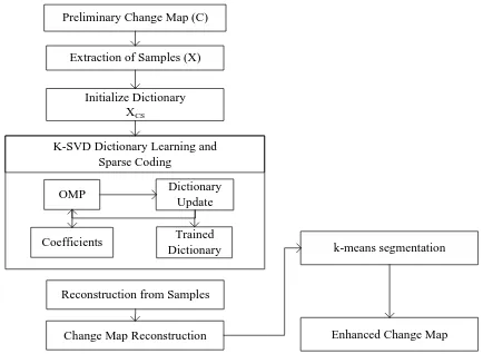
Figure 1. Construction of preliminary change map.
The preliminary change detection map corresponds to the changes obtained from simple differencing of the NDSI/S3 images as shown in Figure 1. NDSI, given in equation 1, is mostly used for snow mapping with multi-spectral satellite imagery (Kulkarni et al., 2002). The reflectance of snow varies differently in visible and shortwave infrared spectrum. The reflectance of snow is higher in case of visible spectrum while lower in shortwave spectrum. Thus it is possible to identify snow using the difference of these two bands from a multi-spectral
Where G and SWIR refer to the reflectance in the green and the shortwave infrared band respectively. In several cases, NDSI may fail to distinguish between snow and water which is often inevitable for studying a glacier in the melt season. The shortwave infrared band allows us to differentiate between snow and water. In the shortwave spectrum the reflectance of snow is much more than water. This aspect could be used to develop a water mask which can then be applied to the preliminary change map. The mask can be created based on the following criteria (Rosenthal and Dozier, 1996)
Identification of the NDSI value (n) for N% of snow covered pixels, say n=50.
Assessing the threshold for the reflectance of water (Iw) relative to the reflectance of snow (Is), say Iw < M%, with M=11%.
Evaluating a pixel as snow, if NDSI value is greater than or equal to n and if Is is greater than M%. However, in our case, such a scenario is barely visible and is thus ignored for simplicity. Identification of snow cover beneath a vegetation canopy is also indefinite due to the similar structure of the spectral reflectance curves for snow and vegetation in the visible and infrared spectrum. In order to identify snow beneath
a forest canopy which is often the case in the Himalayas, the S3 index given in equation 2 could be utilized (Negi et al., 2005).
red and shortwave infrared bands reflectively.3. GENERATION OF ENHANCED CHANGE MAP
3.1 Workflow
Figure 2: Change map enhancement using K-SVD trained dictionary.
The methodology is adopted in a patch based flow, where patches of size 8x8 are extracted for each pixel to generate a sample vector space (one sample corresponds to one column). The extracted samples are formulated into a rectangular matrix of dimensions M x N and sparse coded by compressed sensing with DCT. The resultant compressed samples are used to generate a dictionary which is trained using the K-SVD algorithm. K-SVD is an iterative algorithm for sparse representation of images and their reconstruction. It is widely used in image denoising and can be applied for change detection studies. The change map is reconstructed from sparse decoding and averaging of the patches (samples of the approximation obtained from the K-SVD trained dictionary and coefficients). The developed change map is then segmented using k-means method to differentiate between the changed pixels and non-changed pixels in reference to snow cover.
3.2 Generation of compressed samples
We apply the principle of compressed sensing to construct an initial dictionary which was trained by the K-SVD method. The extracted sample space vectors are compressed using the discrete cosine transform. A dictionary is then generated using this compressed vectors and DCT basis vectors as in equation 3.
.
CS DCT
X DCT X (3)
where DCS is the DCT dictionary (sensing matrix) generated from DCT basis images and compressed vectors XDCT. In general, if a
signal N
XR and a compressed sensing matrix M Nx DR , then Y= DX, where M
YR is the measurements of the signal X. Y, thus sparsely represents the signal X.
3.3 Dictionary learning with K-SVD
For generating a trained dictionary, consider a sample set 1, 2
[ ,...., N]
C c c c corresponding to feature space from compressed sensing, which can be represented as follows
MxK KxN MxN
C D X (4)
where D corresponds to the dictionary to be trained, with atoms 1, 2
CDX is minimum for a sparsely represented X, i.e. maximum X and D that solves the minimization problem. This is carried out in two steps-
1. We can fix the dictionary D and find an approximate set of coefficients �̃. We thus minimize
2 . . 0
X
min CDX s t X t. This is a sparse coding problem with an erroneous solution and can be solved using OMP. OMP is an iterative greedy algorithm, which employs selection of one atom at each step (Rubenstein et al., 2008). The OMP algorithm can be summarized as follows
Import inputs: dictionary D, sparse vectors X, iterations K and the stopping threshold.
a. Initialize counter: t = 1, residual of the norm d. Terminate iteration if stopping condition
2 dictionary that minimizes the norm
2 min CDX such that X 0 kusing the K-SVD approach (Aharon et al., 2006). Using the K-SVD approach the dictionary is updated iteratively with non-zero
coefficients. Since, we update the dictionary atom di, one at each step in a greedy manner, we must consider in our formulation the adjustment of all the rest of the dictionary atoms and coefficients, except those corresponding to the index i. Thus the original minimization problem is now related to the minimization of the error term given as follows
2 2 approximation and Ei corresponds to the error in all N samples while excluding the case when ith atom is anymore. In this case, we may define a group of indices s holding the indices to samples ci corresponding to the non-zero coefficients ofx that employ i di atom. Thus a pointing matrix Oi of size N x s is generated which is sparse. The pointing matrix is used such that is i
i x x O represents a vector of length s with all non-zero entries. Similarly, s
i
c of dimensions N x s corresponds to a sample for the di atom, while E now becomes the is error columns associated to the samples s
i
c . With this in consideration equation 5 can be reformed as in equation 6, which we can minimize using the SVD.
2 2 2
s s i i i i i i i i
E E Od x O E d x (6)
3.4 Reconstruction of the Change Map
The trained dictionary DK-SVD and coefficients
X
ˆ
obtained from the K-SVD algorithm is used to extract the approximate estimates of samples from the change map as given in equation 7.ˆ ˆ
K SVD
CD X (7)
The change map is then reconstructed from columns ofC . The ˆ resultant change map is segmented using the k-means method into two classes, changed pixels in snow cover map and the non-changed pixels. As discussed in section 2, in case of presence of water, the number of classes may be increased. The same is true for vegetation. There are two possibilities to tackle this problem. In the unsupervised approach, we may develop a mask separately for a class. For water we may use the method defined in section 2, otherwise a supervised classification of the enhanced change map could be carried out delivering the changes in multiple classes (Snow, No snow, water, vegetation, etc.).
4. EXPERIMENTS AND RESULTS
To evaluate, the developed methodology, we have experimented with two datasets from Resourcesat-2 and Landsat-8. We use bi-temporal multi-spectral reflectance images to develop the preliminary change maps which is then used for enhancement using the trained dictionary with the KSVD approach. The accuracy assessment was carried out with the kappa statistic. 4.1 Test datasets
The details of the two bi-temporal images from Resourcesat-2 and Landsat-8 used are given in Table 1. These images were downloaded without any cost thanks to Bhuvan, open data archive from the National Remote Sensing Centre (NRSC) and Earth Explorer from the U.S. Geological Survey (USGS) respectively. For experimentation, sections from these images were taken, since the images are relatively large in size. Three tests were performed, using different sections from these images, once with Resourcesat-2 and twice with Landsat-8 (We call these sections as Landsat8a and Landsat8b further). The size of the sections was selected to be around 500x500 pixels, which is ideally suitable for experiments, although Aharon et al., (2006) also provides a model for large image sets. However, this model has not been experimented much with remote sensing images, and still remains computationally rigorous. The test datasets are selected in Himachal Pradesh around the Kalihani glacier (Resourcesat-2), Hadsar village and the Sainj valley (Landsat-8).
Satellite Resourcesat-2 Landsat-8
Date-1 18-10-2008 28-11-2013
Date-2 02-12-2011 02-16-2014
Sensor LISS III OLI-TIRS
Resolution(MSS) 24m 30m
Central region Manali, H.P. Manali, H.P. Table 1. Test datasets
4.2 Generation of the preliminary change maps
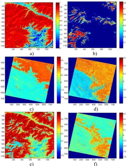
The snow cover maps were generated following the procedure in section 2. The Resourcesat-2 and Landsat-8 images were in 8-bit and 16-bit formats, which were converted to their corresponding reflectance. These reflectance images were used to derive the snow identification indices namely the NDSI and S3. We perform NDSI tests with Resourcesat-2, LISS-III dataset and S3 tests with Landsat-8 OLI imagery. The developed snow cover maps based on the indices as explained in section 2 are shown in Figure 3. The snow cover maps are differenced to obtain a preliminary change map that identifies the regions of changes in snow cover. 4.3 Generation of Enhanced Change Map
The resultant preliminary change map is dissolved into patches of standard size 8 x 8, such that each pixel is represented by a patch, construing a sample space where each column is the sample vector. The sample space is compressed using compressed sensing by multiplication of DCT transformed sample space with a DCT sensing matrix generated from DCT basis images shown in Figure 4. Figure 4b), represents the trained dictionary obtained using the k-SVD approach. This compressed space is used to learn a dictionary using the K-SVD approach. Similar to the patches the dictionary size is defined to be of 64 x 64 to render the computational efficiency optimum. It was noted that increasing the dictionary size requires extremely high
computational efficiency and doesn’t refine the results relatively. We employ Batch-OMP, which is computationally faster than OMP, with a loop stopping threshold. The number of iterations and the acceptable error threshold were set to be 10 and 2 respectively. The averaged coefficients alter very slightly on increasing the number of iterations beyond 10. The dimension L for the sparse coefficients was taken as 10. Increasing the error goal does result in improvements, but at the cost of computational efficiency.
a) b)
c) d)
e) f)
Figure 3. a) & b) NDSI maps for Resourcesat-2 images, c) & d) S3 maps for Landsat-8 images, e) & f) Differences images
generated from NDSI maps and S3 maps respectively.
a) b)
Figure 4.a) DCT basis functions and b) trained K-SVD dictionary for Reourcesat-2 dataset.
For training the dictionary, the K-SVD toolbox by Aharon et al., (2006) was used. The results from the experiment are shown in Figure 5. The change map from the approach in section 3 was post processed by selective histogram thresholds based on the mean and the standard deviation the results. For the Resourcesat-2 dataset, (0.306, 0.Resourcesat-279) are the mean and standard deviations of the result obtained from the approach in section 3, while for the Landsat-8 test datasets (Landsat-8a & Landsat-8b), (0.305, The International Archives of the Photogrammetry, Remote Sensing and Spatial Information Sciences, Volume XL-8, 2014
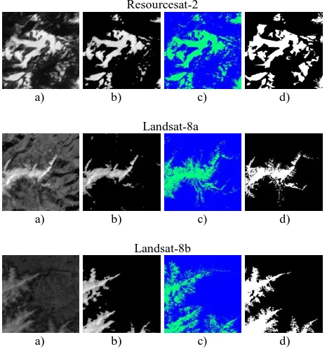
0.158) and (0.334, 0.171) are the mean and standard deviations obtained respectively. The thresholds accurately transformed the change map for k-means classification of 2 classes. The k-means clustering is performed to compare the post classification results with the reference data. In consideration of the changes absolute changes were selected irrespective of being positive or negative to effectively compare against the reference data which is generated by visual interpretation from the difference of the two snow cover maps and the red and shortwave band of the two images. Since the datasets considered, contained relatively lesser water, the water pixels were considered to be the same as the pixels representing land devoid of snow cover. It is possible to identify the water pixels separately from snow, however, for simplicity such a scenario was avoided in experiments. From the results it could be noted that this approach eliminates smaller clusters of pixels from the preliminary change maps. We also perform the supervised classification of the snow cover maps using SVM and difference them for comparison as shown in Figure 5. From the results, it is evident that the differenced SVM classifications approximate the reference data very well. However in the context of several applications like detection of snow cover line, supervised classification are not preferable, since differenced SVM classified maps fail in smoothing the boundaries of the snow accumulation zones.
Resourcesat-2
a) b) c) d)
Landsat-8a
a) b) c) d) Landsat-8b
a) b) c) d) Figure 5. Comparison of the enhanced change map before post
processing (a) and after (b) with the differenced SVM classification (c) and the reference data (d) for the
corresponding datasets.
The accuracy assessment was carried out at pixel level by comparing the k-means classified enhanced change maps with the reference data using the kappa coefficient. The confusion matrix for the three tests performed in this paper are shown in Table 2. Since the overall accuracy from the confusion matrix is not a reliable estimator of accuracy, kappa coefficient was also computed. The obtained kappa coefficient values obtained from our approach are largely acceptable in the Landsat-8 datasets as compared to that of differenced snow cover maps. However, it should be noted that the reference data was generated manually
by visually interpreting the snow cover maps and the red and shortwave reflectance images. Thus the possibly of human error is possible. However, the generated reference data matches the differenced SVM classified maps. The accuracy assessment was also done for the preliminary change map with the reference data. Figure 6 shows the comparison between the obtained overall error and kappa coefficient for the preliminary change map and the enhanced change map.
Resourcesat-2 test dataset k = 0.7, Overall Acc. = 87.1%
Class Change No
Change Total
Prod. Acc.
User Acc. Change 164306 6473 170779 85.75 96.21
No
Change 27306 63547 90853 90.76 69.94 Total 191612 70020 261632
Landsat-8 test dataset-1 k = 0.87, Overall Acc. = 97.5%
Change 23796 286 24082 80.16 8.8
No
Change 5888 220030 225918 99.87 97.39 Total 29684 220316 250000
Landsat-8 test dataset-2 k = 0.8, Overall Acc. = 94.12% Change 35796 12575 48371 94.37 74.00
No
Change 2137 199492 201629 94.07 98.94 Total 37933 212067 250000
Table 2. Accuracy assessment of the approach
Figure 6. Comparison of Overall Accuracy and Kappa Coefficient for the enhanced change map (ECM) and the
preliminary change Map (PCM)
5. CONCLUSION
In this paper, we apply the K-SVD approach for extracting the snow cover changes by improving the preliminary changes The International Archives of the Photogrammetry, Remote Sensing and Spatial Information Sciences, Volume XL-8, 2014
obtained by differencing the snow cover maps. To develop the snow cover maps, we applied NDSI and the S3 index on three different datasets. The K-SVD approach was found extremely efficient in characterizing the accumulation zones of snow cover. In this paper, most of the changes in accumulation zones were reconstructed accurately and were comparable with supervised approaches such as the SVM classification. However, further investigations are necessary to adapt the approach in considering pixels that corresponds to water. Furthermore, the K-SVD approach is computationally challenging. Aharon et al., (2006) does provide a model for increasing the computational runtime of the K-SVD algorithm, which however requires further experimentation with large scale remote sensing datasets. The approach can be effectively utilized for applications which can be modelled with smaller image patches such as monitoring the accumulation zones for a runoff site near a glacier river. The approach can also be applied to monitoring the recession of snow cover line or the changes in glacier area.
6. REFERENCES
Aharon, M., Elad, M., Bruckstein, A., 2006. K-SVD: An Algorithm for Designing Overcomplete Dictionaries for Sparse Representation. IEEE Transactions on Signal Processing 54(11), pp. 4311–4322.
Celik, T., 2009. Multiscale Change Detection in Multitemporal Satellite Images. IEEE Geoscience and Remote Sensing Letters 6(4), pp. 820–824.
Celik, T., 2009. Unsupervised Change Detection in Satellite Images Using Principal Component Analysis and k-Means Clustering. IEEE Geoscience and Remote Sensing Letters 6(4), pp. 772–776.
Fang, L., Li, S., Hu, J. Multitemporal image change detection with compressed sparse representation. 2011 18th IEEE International Conference on Image Processing (ICIP 2011), pp. 2673–2676.
Kulkarni, A.V., Srinivasulu, J., Manjul, S.S., P, M., 2002. Field based spectral reflectance studies to develop NDSI method for snow cover monitoring. Journal of the Indian Society of Remote Sensing 30(1-2), pp. 73–80.
Lu, D., Mausel, P., Batistella, M., Moran, E., 2005. Land‐cover binary change detection methods for use in the moist tropical region of the Amazon: a comparative study. International Journal of Remote Sensing 26(1), pp. 101–114.
Mas, J.-F., 1999. Monitoring land-cover changes: A comparison of change detection techniques. International Journal of Remote Sensing 20(1), pp. 139–152.
Negi, H.S., Mishra, V.D., Mathur, P., 2005. Change detection study for snow covered mountains using remote sensing and ground based measurements. Journal of the Indian Society of Remote Sensing 33(2), pp. 245–251.
Radke, R.J., Andra, S., Al-Kofahi, O., Roysam, B., 2005. Image change detection algorithms: a systematic survey. IEEE Transactions on Image Processing 14(3), pp. 294–307. Rosenthal, W., Dozier, J., 1996. Automated Mapping of Montane Snow Cover at Subpixel Resolution from the Landsat Thematic Mapper. Water Resources Research 32(1), pp. 115–130.
Rubinstein, R., Zibulevsky, M., Elad, M. 2008. “Efficient implementation of the K-SVD algorithm using batch orthogonal matching pursuit,” Technical Report-CS Technion, Jun. 2008. Singh, A., 1989. Review Article Digital change detection techniques using remotely-sensed data. International Journal of Remote Sensing 10(6), pp. 989–1003.