STEREO MODEL SELECTION AND POINT CLOUD FILTERING
USING AN OUT-OF-CORE OCTREE
K. Wenzel, N. Haala, D. Fritsch
Institute for Photogrammetry, University of Stuttgart Geschwister-Scholl-Str. 24D, 70174 Stuttgart, Germany [konrad.wenzel, norbert.haala, dieter.fritsch]@ifp.uni-stuttgart.de
KEY WORDS: Matching, Point Cloud, Photogrammetry, Processing, Integration, Fusion, Sampling
ABSTRACT:
Dense image matching methods enable the retrieval of dense surface information using any kind of imagery. The best quality can be achieved for highly overlapping datasets, which avoids occlusions and provides highly redundant observations. Thus, images are acquired close to each other. This leads to datasets with increasing size - especially when large scenes are captured. While image acquisition can be performed in relatively short time, more time is required for data processing due to the computational complexity of the involved algorithms. For the dense surface reconstruction task, Multi-View Stereo algorithms can be used – which are typically beneficial due to the efficiency of image matching on stereo models. Our dense image matching solution SURE uses such an approach, where the result of stereo matching is fused using a multi-stereo triangulation in order to exploit the available redundancy. One key challenge of such Multi-View Stereo methods is the selection of suitable stereo models, where object space information should be considered to avoid unnecessary processing. Subsequently, the dense image matching step provides up to one 3D point for each pixel, which leads to massive point clouds. This large amount of 3D data needs to be filtered and integrated efficiently in object space. Within this paper, we present an out-of-core octree, which enables neighborhood and overlap analysis between point clouds. It is used on low-resolution point clouds to support the stereo model selection. Also, this tree is designed for the processing of massive point clouds with low memory requirements and thus can be used to perform outlier rejection, redundancy removal and resampling.
1. INTRODUCTION
1.1 Motivation
The first step of Multi-View Stereo methods is the selection of suitable stereo models. This can be achieved using the available orientation information – e.g. the camera position as well as their viewing direction. The viewing direction indicates whether the cameras are convergent or divergent, which can be used to filter suitable stereo models followed by a selection of the n closest cameras.
This approach however suffers from the unknown intersection angles at the object surface, since the distance between the camera and the acquired surface is not known. This is particularly a challenge for short baseline imagery (e.g. video streams), where the intersection angle of the n closest images would be too small to retrieve precise geometry.
Besides, many images cover the same surface and thus highly redundant data is processed. For some applications, this redundancy can be beneficial in order to reduce noise. However, in most applications this benefit does not compensate the high processing time requirements. Thus, a reduction of the involved stereo models would be beneficial, which requires additional knowledge about the geometric conditions.
Consequently, a method is required to analyse the surface in object space – which can be retrieved as a sparse point cloud by performing a dense reconstruction step on low resolution like within our Multi-Stereo solution SURE [Rothermel et al., 2012]. The neighbourhood analysis should be able to detect the overlapping points between point clouds from different images, while automatically adapting to varying point density, as it is frequently occurring due to the varying image scale. Moreover, an option to process large datasets should also be provided to be able to utilize the analysis methods for filtering tasks on high resolution point clouds.
1.2 Stereo model selection for Multi-View Stereo
Stereo model selection is an important step for Multi-View Stereo methods. Besides high coverage, high geometric quality should be achieved. This geometric quality is mainly dependent on image scale and the intersection angle at the object. While a geometrically optimal intersection angle is about 90°, the matching quality suffers from such large intersection angles, since the image similarity is low. This leads to lower performance for image matching and thus to lower reliability and density. This is particularly to be considered for dense matching tasks, which yield high completeness at the surface.
Besides the intersection angle, the image similarity is decreased for surfaces, which are not parallel to the image plane. Furthermore, such slanted surfaces are particularly difficult for dense matching algorithms similar to Semi Global Matching as used in SURE, due to the smoothness constraint used in these algorithms [Wenzel et al., 2013]. This smoothness constraint is based on penalty terms, where disparity jumps of zero or one pixel are treated with a lower penalty than higher jumps. Thus, the optimization through the smoothness constraint gets lost if a disparity gradient of 1 is exceeded.
Apart from image similarity and matching performance, the mutual coverage of stereo models is also decreased with higher intersection angles – in particular for non-planar objects. Within previous investigations, stereo models between 5 and 30 degree intersections have shown to be a suitable compromise for arbitrary surfaces [Wenzel et al., 2013]. In particular when multi-stereo triangulation like in SURE is used, such intersection angles can lead to high geometric quality if the cameras are well distributed. For example, an image with one stereo model on the left side with 20 degrees and another model on the right side with 20 degrees leads to an overall intersection angle of 40 degrees for pixels that could successfully be matched in both stereo models. At the same time, the image similarity within the stereo models is high, which leads to a high matching quality.
A simple approach to stereo model selection is the selection based on the n closest stereo models to a particular image. This approach however fails, if the image density is very high (e.g. video) or the distance to the object is high – since both lead to too low intersection angles at the object and thus to insufficient precision on the object.
In order to improve stereo model selection, object space information should be taken into account. The selection should be performed according to suitable intersection angles at the object, while taking the overlap into account since it indicates connection as well as mutual coverage of each particular stereo model. Thus, completeness and geometric quality can be improved.
1.3 Approach
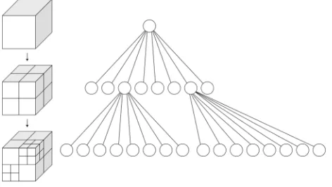
In order to perform overlap analysis in object space, nearest neighbourhood analysis needs to be performed efficiently. Such efficient queries can be implemented using indexing and tree structures, such as the octree data structure [Meagher et al., 1980], which indexes the data by subsequently partitioning a cube into eight sub-cubes. Octrees also support efficient data update and are suitable for out-of-core implementations - enabling streaming data from the hard disk, instead of keeping the entire data in the main memory. Thus, only the currently required data is held in the memory, while unused parts are written to disk.
Out-of-core tree structures are widely used – in research often for visualization, such as [Ueng et al., 1997], [Corrêa et al., 2002] or [Lindstrom, 2003]. Besides this application, processing on the data is also performed – for example Poisson surface reconstruction like in [Bolitho et al., 2007] or mesh simplification [Cignoni et al., 2003]. [Elseberg et al., 2011] use an out-of-core tree with adaptive depth also for point cloud processing and visualization, which improves the support of non-uniformly distributed point clouds.
For the tasks of overlap analysis and point cloud filtering, we require a flexible implementation of such an out-of-core
structure, enabling specific operations on tree nodes as well as additional data fields. Within this paper, we use the PineTree
implementation, which we presented in[Wenzel et al., 2014]. The Pine Tree framework is based on an octree, and thus allows fast data adding and update. Its regular spatial driven portioning can be implemented efficiently for operations in-core, but also enables switching to out-of-core storage for parts of the tree if required.
In order to perform the selection of suitable images as well as the stereo models, the information of overlapping surfaces is required. For this purpose, one point cloud is derived for each image using dense image matching on low resolution (e.g. 200 by 200 Pixels). Subsequently, the tree is subdivided into deeper levels, until each node contains not more than a predefined count of points of each point cloud. This leads to clusters of
homologous points indicating overlap information independent of the scale and adapting to non-uniform distribution and density.
Within the analysis of overlap in object space, this overlap information can be used to build connectivity information. This connectivity information is subsequently analysed to select stereo models and images to be processed in order to improve the geometric quality of the reconstruction and to reduce processing time.
Fig. 1: Octree data structure for spatial indexing. The space is subsequently partitioned into eight equal sized sub-cubes. At the final nodes, the data is stored – enabling fast neighbourhood queries by
top-down tree traversal. Image source: Wikipedia
The retrieval of homologous points is also beneficial for the task of point cloud filtering. It can be customized to spatial resampling using a pre-defined minimum voxel width or a specified reduction-factor of the local resolution. The latter also adapts to non-uniform distribution.
Besides the reduction of redundancy and spatial resampling, an outlier rejection can be performed since noisy points from more sparse clouds (e.g. due to other image scale) will not be included in this voxel. This can be complemented by an additional constraint of a minimum number of detections from different clouds, which enables validation in object space.
Within this paper, the stereo voxel partitioning on multiple clouds – including the determination of homologous points for the overlap estimation and the point filtering approach, will be described in section 2. The homologous point information serves as a base for the overlap analysis for the determination of suitable images and stereo models, which is described in section 3. In section 4, the performance of the presented approach is discussed in respect to exemplary datasets – followed by the conclusions and future work in section 5.
2. VOXEL PARTITIONING ON MULTIPLE CLOUDS
2.1 Determination of homologous points
For point clouds from images – e.g. derived using dense image matching methods, the source image is known for each point. This information can be used for further analysis, such as local density estimation, redundancy detection or overlap information determination in object space. In order to derive this information, identical points between the point clouds
(homologous points) need to be detected.
The key challenge of point clouds from image matching is the non-uniform distribution, which is mainly caused by varying image scale. Thus, we always consider the densest point cloud as a reference. A point is homologous to another point in this densest point cloud, if it is with half of the distance to the closest point of the densest point cloud. Thus, each point needs to be evaluated with respect to its neighbourhood – in particular, the locally densest point cloud. In order to provide an efficient implementation, we use the native voxel shaped tree structure of the octree used in the PineTree framework, to perform an approximated nearest neighbour query. Thus, we evaluate voxel cubes and its sub-partitions instead of evaluating each point individually, enabling more efficient processing.
2.2 Filtering based on point source information
2.2.1 Filtering locally densest cloud
After adding point clouds from multiple images to the octree data structure, the partitioning can be used to evaluate the local neighbourhood based on constraints on this point source information. This enables adaptive approaches guided by the locally densest cloud, instead of defining a fixed tree depth or a fixed voxel width.
By constraining each voxel to have only one point from each source, the partitioning of the tree will be performed until each final voxel has the width according to the highest point density. By rejecting all other point clouds, only the densest cloud is preserved, which is typically the one with the highest precision. Alternatively, other measures of precision can be used as constraint if available. The filtering is thus particularly beneficial to reduce redundancy by preserving only precise information.
2.2.2 Point validation
Furthermore, adding a constraint of having at least two points in this voxel, a validation of this point can be performed. If no additional point from another source is available, the points in the voxel are rejected, otherwise the remaining points can either be merged or only the point from the locally densest cloud is preserved. Enforcing such a fold constraint enables validation in object space, where each point needs to be confirmed by a point from another point source. Thus, outliers can be rejected. This is beneficial, when images are covering the same object, but are not suited for image matching between each other - e.g. due to a too large baseline or different image scale. Here, surface information can be derived for each image cluster by performing stereo matching on suitable models, followed by integration in object space of the resulting point clouds.
2.3 Extended voxel sizes
In the default approach, the tree is sub-partitioned, until each voxel has only one point from each image-wise point cloud and thus, adapts to the locally densest cloud. This approach can also be extended by setting the threshold of this maximum occurrence of each class in a voxel to higher values than 1. For example, with a threshold of 4, data reduction can be performed adaptively, since 4 points of the densest cloud will be merged to one cloud.
Besides the adaptive voxel size, constraints for a fixed voxel width can also be introduced, where the sub-partitioning is performed until either the maximum occurrence threshold or this fixed voxel size is reached. This leads to equally distributed points where sufficient data density is available.
3. STEREO MODEL SELECTION
3.1 Stereo model selection in object space
As stated in section 1.2, a suitable stereo model selection should ensure for each stereo model
1) Sufficient overlap between the stereo models, in order to ensure completeness and image similarity.
2) A sufficient intersection angle at the object, in order to optimize the geometric condition for precision.
3.1.1 Object space information
In order to retrieve the intersection angle at the object, object space information is required. If no prior information is given (e.g. sparse feature points from Structure from Motion), this information can be retrieved using Dense Image Matching at low resolution (e.g. 200 by 200 pixels). For each decreased resolution level, the image resolution is decreased by a factor of 4, while the disparities to be evaluated decrease by a factor of 2 like the image width. Thus, each lower resolution level decreases the complexity of the matching by 1/8 – which results for a level 5 processing in a 1/40th of the processing time at original resolution. Consequently, one low resolution point cloud per image can be derived efficiently, which can be analysed within subsequent steps.
3.1.2 Overlap estimation
The estimation of overlap in object space is performed using the sparse point clouds derived from the previous step. Given that one point cloud is derived for each image, the clouds can be integrated into an adaptive voxel grid as described in section 2. Here, the used octree is sub-partitioned, until each voxel contains a maximum of one point per point cloud. By enforcing a minimum number of points from several clouds (e.g. fold 2), data filtering can be performed as described in section 2.2.2.
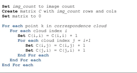
As a result, each integrated point can be stored with its corresponding point source information, stored as a vector of cloud indices for each point. This correspondence cloud can then be used to derive a connectivity matrix – indicating the number of connections for each stereo model. In order to derive this matrix, one connection is added for each correspondence of different clouds for each point in the correspondence cloud, as shown in table 1.
Set img_count to image count
Create matrix C with img_count rows and cols Set matrix to 0
For each point k in correspondence cloud
For each cloud index i
Set C(i,i) = C(i,i) + 1
For each cloud index j = i+1
Set C(i,j) = C(i,j) + 1 Set C(j,i) = C(j,i) + 1 End For each
End For each End For each
Table 1: Derivation of connectivity matrix from correspondence cloud
The result from this step is a connectivity matrix C, indicating the number of connections for each stereo model (point count connectivity). The count of points for the stereo model between image i and image j can be found in the matrix element C( i, j ). On the main diagonal, the total number of points with connections for this image can be found. Thus, a normalized point count connectivity can be created, by dividing each row r by its total number of points on the diagonal element C( i, j ).
Consequently, each element value in each row r depicts the percentage of connections and thus, the overlap in object space. By using a maximum occurrence of 1, the voxels are partitioned until only one point from each point cloud is available. However, this voxel width is typically too small to derive reliable overlap information, due to shifts of the point clouds, density differences and sampling effects from the voxel grid.
Consequently, the voxel width for deriving the correspondence point cloud needs to be extended. As described in section 2.3, the voxel width can be extended by either defining a minimum voxel width value, or by increasing the maximum occurrence threshold. However, the first approach doesn’t adapt to non-uniform distribution – furthermore, the desired sampling width is typically not known. Thus, we use an increased maximum occurrence value (e.g. 10), which leads to clusters of points. Since each correspondence within such a cluster is only taken into account once, the correspondence information becomes more reliable. Furthermore, the number of correspondences is reduced, which is beneficial for processing time in particular for large datasets.
3.1.3 Angle estimation
In order to estimate the angle between stereo models, the angle of intersection at each point from the correspondence point cloud is evaluated. For this purpose, two rays are reconstructed from the known camera centres of the respective images to this point. With the cosine function, the angle between these rays can be determined. This angle is stored in another connectivity matrix similar to section 3.1.2, where each stereo model between image i und j is represented in the matrix cell i, j. In order to derive the mean angle for each stereo model, the angles are accumulated by adding up the angles determined for each model in the respective cell in the angle connectivity matrix A.
3.1.4 Decision criterion
Stereo models with long baselines for optimal intersection angles typically suffer from insufficient overlap and image similarity. In contrast, stereo models with short baseline and optimal image similarity, typically suffer from an insufficient intersection angle. Thus, a compromise is required to select the optimal stereo model.
For this purpose, we propose a combined criterion – comprising the overlap and a mean angle at the object. The value is represented in the normalized point count connectivity described in section 3.1.2, which indicates the overlap within a range between 0 and 1. The mean angle is available in the angle connectivity matrix.
The algorithm shall select stereo models closest to a certain angle, while taking into account the overlap information. For this purpose, a vector of desired angles can be defined (e.g. 10° and 20°) to derive stereo models close to this configuration. In order to avoid rough thresholds but to adapt flexibly, we use a Gaussian distribution around the defined angles as weight for the overlap information. This results in a decision criterion.
The Gaussian distribution can be represented by the probability density function depending on the parameter x, an expectation
For our purposes, we require a distribution with a value range of [0,1] dependent on the desired angle (e.g. the selected 10°) according to the given angles . For this purpose, we omit the normalization and define the distribution with regard to the given angles. Furthermore, we add a small constant shift (e.g. 0.01), to not let the distribution be close to 0, but allow small weights for stereo models distant to the desired angle. This is beneficial, if no other stereo models are available.
Introducing the shift requires again normalization, in order to achieve a value range for the angle weight between 0 and 1.
In order to prefer images with high overlap and similar angles at once, we can integrate the overlap with the angle weight to the previously determined vector of angles . For example, two stereo models with 15° can be determined iteratively, by deactivating already selected models.
A key parameter of the criterion is now the standard deviation, since it defines the allowed range, where the angle overrules the overlap information. For example, if a stereo model of 5° is selected, but another model with 8° degrees exists with a 50% higher overlap, we would like to allow the decision to prefer the more overlapping image. For this purpose, we select a rather high standard deviation (e.g. 10 degrees) – enabling a rough preference, while not overruling the important overlap information.
For equally distributed stations – e.g. as a circle around an object, the algorithm would select the left and right image. Furthermore, the weighting of the angle enables the selection of a stereo model even if no model with the desired angle exists. It will be selected according to the angle similarity and the available overlap. This enables the specification of generic angles , where the impact of the angle in relation to the overlap is defined by . At a difference of one to the selected angle, the proposed distribution will lead to a weight of roughly 0.5, and thus compensates at this point a 50% higher overlap of the image. Closer to the selected angle µ, stereo models with higher overlap will still be preferred, since the weight difference is smaller.
3.1.5 Implementation overview
The implementation of the stereo model selection can be divided into the following steps:
1) Overlap estimation:
a. Integration into voxel space
b. Building up of correspondence point cloud 2) Derivation of point count connectivity matrix
a. Normalization (contains )
3) Derivation of angle connectivity matrix (contains ) 4) Determination of suitable models
For each image i:
For each desired angle :
- Determine decision criterion (,) - Find and select maximum of - Deactivate model for following queries
4. DISCUSSION
The proposed method for stereo model selection and point cloud filtering has been shown for three exemplary datasets on pages 6-8.
The first dataset consists of 43 camera stations acquired as a ring around a church ruin in St. Andrews, Scotland. Thus, the angle between each image is roughly 8-10 degrees. For evaluation purposes, we defined the angles to be selected (µ) as two 8 degree models, two 16 degree models and two 32 degree models – even though such a large amount of stereo models would in practice not be required. Figure 2.2 shows the normalized overlap connectivity matrix, which indicates the connection in dependency of the area covered by the particular image. Furthermore, the mean angle connectivity as well as the finally selected stereo models are shown. The selected stereo models show that the selection according to the angle succeeds. In the following figure 2.3, the overlaps as well as the decision criterion for selection is given, where the overlap is weighted with the selected angle. Figure 2.4 shows the result of dense surface reconstruction with SURE. The filtering described in section 2.2 was applied using different values for the maximum occurrence value. As shown, the data amount can be reduced while preserving detail.
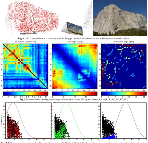
The El Capitan example on page 7 shows a dataset from Yosemite National Park in California. 42 images were acquired with wide angle and far distance from a large object. The key challenge in this dataset is the small baseline between the images with respect to the distance to the object. For the classical approach of selecting n nearest neighbours (e.g. 5) as the stereo model, the dense reconstruction would lead to unreliable data due to insufficient geometric conditions. The presented approach selects the models based on the object space information and enables the derivation of a reasonable surface.
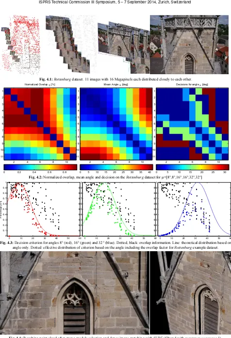
The Rottenburg example on page 8 shows a partial dataset of a church tower, which was acquired using an octocopter RPAS. Here, the challenge is the inhomogeneous distribution including very short base lines between the first images. Also here, the algorithm proofs to select the right stereo models according to the specified angles.
5. CONCLUSIONS AND FUTURE WORK
The out-of-core octree used within this work proved as a suitable solution for spatial data storage and querying. Due to the out-of-core technique, not the whole datasets needs to be in memory, but can be processed automatically in parts. This enables scalability to large datasets. Furthermore, the octree represents a tree structure suitable for fast data queries, while supporting efficient data update and removal. Within Multi— Stereo methods for dense surface reconstruction, this enables processing surface information in object space. This is suitable for a variety of applications, such as point cloud filtering as described in section 2, but also for stereo model selection as described in section 3.
For the point cloud filtering, the tree is used in combination with constraints on the point source information resulting from different point clouds. By partitioning the tree until each voxel contains only one point from each point cloud, the point cloud with the highest local density can be filtered. This is particularly beneficial for Photogrammetric applications, where the varying image scale leads to non-uniform point distribution. Furthermore, constraints on minimum detections from different sources can be used to perform point validation in object space.
Within the stereo model selection, the flexible structure of the tree can be used to analyse overlaps between point clouds efficiently. Adaptive voxel sizes enable a clustering adapting to the local point density, while providing reliable overlap
information. In order to determine optimal stereo models, this overlap and the local intersection angle are taken into account using a weighting function. The resulting criterion can be maximized to find suitable stereo models according to predefined intersection angles, while the method adapts robustly by selecting alternative models if models with the particular angles are not available.
The presented approach can be reduced to improve geometric conditions for the dense reconstruction, but also to reduce processing time. This is in particular suitable for datasets, where images were acquired with small baselines – e.g. due to high acquisition frequency as found in video streams.
Within future work, the impact of different configurations of selected angles will be further evaluated. Furthermore, the image point clouds will be evaluated in clusters according to the depth, in order to avoid difficulties of the mean angle due to large depth variations in the scene. Also, the derived overlap information shall be used to determine a minimum set of reliable stereo models, in order to reduce processing time.
6. REFERENCES
Bolitho, M., Kazhdan, M., Burns, R., & Hoppe, H. (2007, July). Multilevel streaming for out-of-core surface reconstruction. In Symposium on geometry processing (pp. 69-78).
Cignoni, P., Montani, C., Rocchini, C., & Scopigno, R. (2003). External memory management and simplification of huge meshes. Visualization and Computer Graphics, IEEE Transactions on, 9(4), 525-537.
Corrêa, W. T., Klosowski, J. T., & Silva, C. T. (2002). iWalk: Interactive out-of-core rendering of large models. Technical Report TR-653-02, Princeton University.
Elseberg, J., Borrmann, D., & Nuchter, A. (2011). Efficient processing of large 3d point clouds. In Information, Communication and Automation Technologies (ICAT), 2011 XXIII International Symposium on (pp. 1-7). IEEE.
Lindstrom, P. (2003, April). Out-of-core construction and visualization of multiresolution surfaces. In Proceedings of the 2003 symposium on Interactive 3D graphics (pp. 93-102). ACM.
Meagher, D. J. (1980). Octree encoding: A new technique for the representation, manipulation and display of arbitrary 3-d objects by computer. Electrical and Systems Engineering Department Rensseiaer Polytechnic Institute Image Processing Laboratory.
Rothermel, M., Wenzel, K., Fritsch, D., Haala, N. (2012). SURE: Photogrammetric Surface Reconstruction from Imagery. Proceedings LC3D Workshop, Berlin, December 2012.
http://www.ifp.uni-stuttgart.de/publications/software/sure/index.en.html
Ueng, S. K., Sikorski, C., & Ma, K. L. (1997). Out-of-core streamline visualization on large unstructured meshes. Visualization and Computer Graphics, IEEE Transactions.
Wenzel, K., Rothermel, M., Fritsch, D. & Haala, N. (2013). Image Acquisition and Model Selection for Multi-View Stereo, Int. Arch. Photogramm. Remote Sens. Spatial Inf. Sci., XL-5/W1, 251-258, 2013.
Wenzel, K., Rothermel, M., Haala, N. & Fritsch, D. (2014). Filtering of Point Clouds from Photogrammetric Surface Reconstruction. Int. Arch. Photogramm. Remote Sens. Spatial Inf. Sci., XL-5-615-2014
Fig. 2.1: St. Andrews dataset. 43 images with 5 Megapixels each distributed in a circle around the object.
Fig. 2.2: Normalized overlap, mean angle and decision on the St. Andrews dataset for µ=[8°,8°,16°,16°,32°,32°]
Fig. 2.3: Decision criterion for angles 8° (red), 16° (green) and 32° (blue). Dotted, black: overlap information. Line: theoretical distribution based on angle only. Dotted: effective distribution of criterion based on the angle including the overlap factor for St. Andrews example dataset.
Fig. 2.4: Resulting point cloud after stereo models selection and dense image matching with SURE. Left: full view, filtered with maximum occurence
1. Right: Detail from full cloud (49.1 Mio. pts.), filtered with mo 1 (7.1 Mio. pts.), filtered with mo 2 (3.8 Mio. pts.), filtered with mo 4 (1.9 Mio. pts.)
Normalized Overlap η [%]
5 10 15 20 25 30 35 40 5
10
15
20
25
30
35
40
0 0.1 0.2 0.3 0.4 0.5 0.6 0.7 0.8 0.9
Mean Angle α [deg]
5 10 15 20 25 30 35 40 5
10
15
20
25
30
35
40
20 40 60 80 100 120 140 160
Decisions for angle µ [deg]
5 10 15 20 25 30 35 40 5
10
15
20
25
30
35
40
0 5 10 15 20 25 30
0 10 20 30 40 50 60
0 0.1 0.2 0.3 0.4 0.5 0.6 0.7 0.8 0.9 1
P
e
rc
e
n
ta
g
e
[
0
:1
]
0 10 20 30 40 50 60
0 0.1 0.2 0.3 0.4 0.5 0.6 0.7 0.8 0.9 1
0 10 20 30 40 50 60
0 0.1 0.2 0.3 0.4 0.5 0.6 0.7 0.8 0.9 1
Fig. 3.1: El Capitan dataset. 42 images with 16 Megapixels each distributed in line at far distance from the object.
Fig. 3.2: Normalized overlap, mean angle and decision on the El Capitan dataset for µ=[8°,8°,16°,16°,32°,32°]
Fig. 3.3: Decision criterion for angles 8° (red), 16° (green) and 32° (blue). Dotted, black: overlap information. Line: theoretical distribution based on angle only. Dotted: effective distribution of criterion based on the angle including the overlap factor for El Capitan example dataset.
Fig. 3.4: Left: resulting point cloud after stereo models selection and dense image matching with SURE. Right: triangle mesh derived from point cloud. Point cloud count original: 146 Mio. pts. Filtering with maximum occurrence 1: 31 Mio. pts., mo 2: 18 Mio. pts., mo 4: 11 Mio. pts.
Normalized Overlap η [%]
5 10 15 20 25 30 35 40
5
10
15
20
25
30
35
40
0 0.1 0.2 0.3 0.4 0.5 0.6 0.7
Mean Angle α [deg]
5 10 15 20 25 30 35 40
5
10
15
20
25
30
35
40
0 5 10 15
Decisions for angle µ [deg]
5 10 15 20 25 30 35 40
5
10
15
20
25
30
35
40
0 5 10 15 20 25 30
0 10 20 30 40 50 60
0 0.1 0.2 0.3 0.4 0.5 0.6 0.7 0.8 0.9 1
P
e
rc
e
n
ta
g
e
[
0
:1
]
0 10 20 30 40 50 60
0 0.1 0.2 0.3 0.4 0.5 0.6 0.7 0.8 0.9 1
0 10 20 30 40 50 60
0 0.1 0.2 0.3 0.4 0.5 0.6 0.7 0.8 0.9 1
Fig. 4.1:Rottenburg dataset. 11 images with 16 Megapixels each distributed closely to each other.
Fig. 4.2: Normalized overlap, mean angle and decision on the Rottenburg dataset for µ=[8°,8°,16°,16°,32°,32°]
Fig. 4.3: Decision criterion for angles 8° (red), 16° (green) and 32° (blue). Dotted, black: overlap information. Line: theoretical distribution based on angle only. Dotted: effective distribution of criterion based on the angle including the overlap factor for Rottenburg example dataset.
Fig. 4.4: Resulting point cloud after stereo models selection and dense image matching with SURE (filtered with maximum occurence 1). Full cloud (84 Mio. pts.), filtered with mo 1 (13 Mio. pts.), filtered with mo 2 (5 Mio. pts.), filtered with mo 4 (2.4 Mio. pts.)
Normalized Overlap η [%]
2 4 6 8 10
1 2 3 4 5 6 7 8 9 10 11
0 0.2 0.4 0.6 0.8
Mean Angle α [deg]
2 4 6 8 10
1 2 3 4 5 6 7 8 9 10 11
0 5 10 15 20 25 30 35 40
Decisions for angle µ [deg]
2 4 6 8 10
1 2 3 4 5 6 7 8 9 10 11
0 5 10 15 20 25 30
0 10 20 30 40 50 60
0 0.1 0.2 0.3 0.4 0.5 0.6 0.7 0.8 0.9 1
P
e
rc
e
n
ta
g
e
[
0
:1
]
0 10 20 30 40 50 60
0 0.1 0.2 0.3 0.4 0.5 0.6 0.7 0.8 0.9 1
0 10 20 30 40 50 60
0 0.1 0.2 0.3 0.4 0.5 0.6 0.7 0.8 0.9 1