SWEEPING RASTER CROSS SECTIONS ALONG TRAJECTORIES
IN THREE-DIMENSIONAL VOXEL MODELS
Ben Gorte1*, Sisi Zlatanova2, Alan Leidner3
1Dept. of Geoscience and Remote Sensing, 2Dept. of Urbanism, Delft University of Technology, the Netherlands
[email protected], [email protected] 3
New York Geospatial Catalysts (NYGEOCATS), [email protected]
Commission IV
KEY WORDS: Sweeping, voxelization, 3D grid, underground infrastructure model
ABSTRACT:
The paper presents a new algorithm to reconstruct elongated objects defined by cross sections and trajectories in gridded three-dimensional models represented as voxels. Examples of such objects are the elements of underground infrastructure in urban environments, such as pipes, conduits and tunnels. Starting from a basic methodology, which is based on distance transformations, the algorithm is extended in three ways on the basis of Voronoi datasets being produced alongside.
1. INTRODUCTION
The importance of the underground infrastructure in a modern urban environment can hardly be over-estimated. Thousands of kilometers of cables, pipes, ducts and conduits are located below the street surface of any major city, supporting transport and distribution of electricity, gas, fresh water, waste water, and signals for telecommunication (such as telephone, cable TV and internet), along with manholes and tunnels to provide access for maintenance and repair. Having good descriptions of the various sorts of infrastructure seems vital to the companies and agencies involved, whereas an integration of the different datasets will support planning, preparation and execution of any kind of installation and maintenance work. In addition, having integrated infrastructure information available will be vital in case of emergencies, such as floods, landslides, earthquakes and accidents.
When creating and integrating underground infrastructure information, it is obviously difficult to make new measurements (Birken e.a., 2002), whereas the existing information tends to be scattered among the various parties involved. Moreover it should be acknowledged that free availability of detailed and integrated underground infrastructure information involves a vulnerability risk for an urban society. Therefore, setting up such information requires flexibility at the side of the input (when dealing with heterogeneous and scattered data sources), as well as on the side of the output (when choosing levels of detail, both geometrically and semantically).
Fortunately, many elements of underground infrastructure, such as conduits and tunnels, have elongated shapes, which can be adequately described by a cross section and a trajectory. In this paper we investigate 3d reconstruction of models on the basis of exactly these two data sources, which exist in the databases of the underground infrastructure and utility organisations for construction and maintenance purposes.
The final objective of the project at hand is to combine underground infrastructure models with continuously-varying surrounding soil parameters such as moisture, salinity,
pollutants etc. Therefore, we are aiming to integrate all the information in a unified voxel representation. We believe this approach may enable resolving spatial conflicts easily and allow for various types of spatial computations such as 3d distances, volumes and cross sections, or determining 3d topological and other spatial relationships, which seem problematic in vector domain. Furthermore, modelling volumetric objects, such as underground, water, walls, air requires the deployment of complex shapes, which are prone to validity errors. We are aware that the choice of representing spatial information (notably geo-information) in raster form, both in two and three dimensions, is not undisputed. Entering this discussion, however, is not the goal of this paper. The purpose of this effort, is to investigate direct raster algorithms for 3d reconstruction of certain objects.
1.1 Sweeping
The goal of the algorithm we are presenting is commonly referred to as sweeping. In the field of Constructive Solid Geometry (CSG) within Computer Graphics sweeping is a way to describe a three-dimensional primitive volume in terms of a two-dimensional profile shape (a cross section of the volume) and a trajectory (a line or curve in 3d space along which the volume extends). The primitive is defined as the set of all points that are ‘hit’ by the profile shape when it moves along the trajectory. The moving shape is kept perpendicular to the trajectory, but other than that, the shape is not rotating – it is kept as “upright” as possible, within the perpendicularity constraint (translational sweep) (Foley et al., 1996).
Sweeping has been implemented in the vector domain, for example in CAD programs, where it may be performed interactively and results in a volumetric object bounded by a polyhedral mesh. Sweeping is also described in the raster (voxel) domain, for example in (Chen et al. 2000), which however does not provide an implementation. A possible raster implementation is obviously to perform the above-mentioned vector sweep, followed by a solid rasterization of the resulting polyhedron (Nooruddin and Turk, 2003, Eisemann et al, 2008, or Gorte and Zlatanova, 2016). We want to address a direct raster sweep, however, where the profile shape is given as a
2D raster “image” (Fig. 2 below) and also the trajectory consists of a (thin, elongated, either straight or curved) set of voxels (Fig. 3).
An issue in direct raster approaches is that whenever the trajectory is not exactly aligned with one of the coordinate axes, the profile shape has to be re-sampled into the voxel space. When, in addition, the direction of the trajectory is varying, because the trajectory is curved or bended, then so is the transformation between input pixel coordinates and output voxel coordinates used in the re-sampling. In such cases it is inevitable that some of the affected output voxels are ‘hit’ multiple times, possibly even with different pixels (having different values or semantics, between which a choice has to be made), whereas other voxels are ‘missed’ in the process, leaving holes in the resulting 3d object (Fig. 1). This has to be repaired by over-sampling, interpolation and/or anti-aliasing. We will present hereafter a new, output driven, direct raster sweeping algorithm, which has the advantage that every
participating output voxel receives its (correct) value only once.
Figure 1: Multiple assignments and holes in input driven raster sweep
In an attempt to make the text less abstract, we will first show the input and the result of the basic algorithm and describe its principle, before explaining how it works in detail in section 3. In section 4 we will introduce a number of refinements, which have in common that they are based on Voronoi images.
2. THE GOAL
We present an algorithm that takes as its input a raster representation of the cross section of an elongated underground construction (Fig. 2), as well as a rasterized 2d curve that marks the trajectory along which the construction extends (Fig. 3). The result of the algorithm is a voxel space in which the cross section is extruded (‘swept’) along the trajectory (Fig. 4).
Figure 2: Raster image of the cross section of a subway station. The height of the cross-section gives the height of 3d voxel
space
Figure 3: Trajectory of the subway station. The size of the trajectory image determines the horizontal extend of the 3d
voxel space
It is assumed that the cross section (Fig. 2), as well as the trajectory, are already rasterized in the target resolution of the voxel dataset (0.25m in all examples in this paper). Therefore, the horizontal extent of the voxel dataset is given by the size of the trajectory grid, and its height by the cross section height.
The purpose of the algorithm is to fill a voxel ‘block’ V, whose dimensions are given by the trajectory image (horizontally) and the cross section image (vertically), with values from the cross section image C. We need a mapping from 3d coordinates (x,y,z) to cross section coordinates (u,v), to be able to execute
V[x,y,z] = C[u,v] (1)
for all x,y,z in V. Also see Section 3.
Figure 4. The resulting 3d voxel space with object voxels in blue and background voxels in grey.
An anchor point (u0,v0) is given in C (Fig 7, right), as well as signed, perpendicular distances in trajectory images next.
3.1 Cross sections
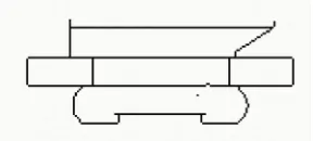
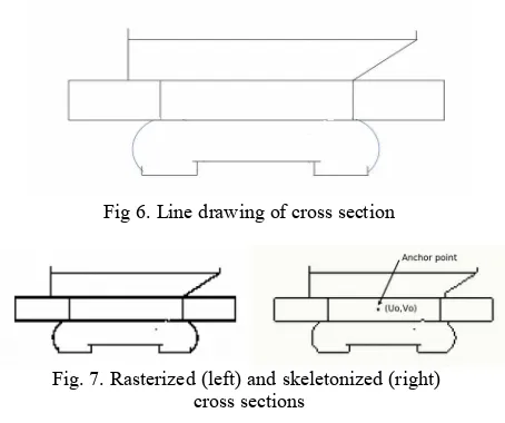
A picture of a subway station (in Melbourne, AUS, Fig. 5) was found on the Internet and used as a basis for on-screen identification of the important elements (floors, walls and ceilings). The resulting line drawing (Fig. 6) was rasterized to an estimated 25cm resolution and skeletonized (Serra, 1988) (Fig. 7) – the latter step is optional, but is sensible under the assumption that all relevant elements are adequately represented at a single voxel thickness.
Fig 6. Line drawing of cross section
Fig. 7. Rasterized (left) and skeletonized (right) cross sections
The cross section in Fig. 7 is binary, having only object (black) and background (white) values. Our method can easily be
The cross section pixels have integer (u,v) coordinates for their horizontal and vertical positions, respectively. The indicated anchor point is the coordinate (u0,v0) of the point in the cross section image that will exactly follow the trajectory during the sweep (Fig. 7 right).
3.2 Resampling
During the sweep we fill a block of voxels V with values from a cross section image C. For this we have to establish a relation between (x,y,z) coordinates in V and (u,v) coordinates in C. In a way the problem resembles classical image
resampling, which, for example, is used in geometric correction of Remote Sensing imagery. Here the objective is to copy pixel values (densities, radiances, or reflectrances) from locations (u,v) in an input image I to new locations (x,y) in an output image O, given a geometric transformation T that links the two coordinate systems: (x,y) = T(u,v). In some applications this process is also known as warping, in others as morphing.
The input-driven (or direct) resampling method traverses the input image and uses T to compute at each input pixel the location at which its value has to be put in the output image. The output driven (or indirect) method needs the inverse transformation T -1, which gives (u,v) = T -1 (x,y). It traverses the entire output image and computes at each output pixel the location in the input from which the value has to be taken (Konecny, 2003).
The input driven method has the disadvantage that T may yield non-integer (x,y) coordinates from integer (u,v). The question the becomes where to put a value when the computed location (x,y) = (456.43,130.66). Moreover it may happen that certain output locations are targeted more than once (probably with different decimal fractions) when the image is being spatially compressed, whereas other output locations are not reached at all, when the image is being expanded. Post-processing may overcome those disadvantages, but the important observation is here that output driven method does not have them! If the (integer) output coordinates (x,y) transform into fractional input coordinates (u,v), then interpolation can be easily applied on-the-fly (e.g. nearest neighbour, bilinear interpolation or cubic convolution). Moreover, every output pixel will obtain one and only one value. For completeness we notice that the choice between the input and the output driven method also depends on the availability of T and T -1.
We will develop voxel sweep in an output driven (“indirect”) way, using a transformation that gives for every (x,y,z) coordinate in the voxel space V exactly one (u,v) coordinate in the cross section image C. This transformation would have the role of T -1 in the above formulation.
Note that this transformation is not necessarily expressed in a single formula. Besides, “our” transformation cannot be easily inverted; for a direct method one would have to follow a different approach. An obvious attempt would be to define and construct planes in the voxel space, perpendicular to the trajectory. This, however, requires the trajectory’s (local) direction, which may be not easily established when it only exists as a set of voxels. Also because of the above-mentioned other, more general, issues of input-driven methods we will not pursue this any further here.
The voxel space V can be considered a stack of rectangular slices, each having a one voxel thickness. The voxels inside a slice have (x,y) coordinates, and each slice has a z coordinate. Initially V is empty (every voxel has the nodata value), except for one slice at z0 that contains the trajectory image of Fig. 3. The trajectory is a simple, connected, thin (skeletonized, as mentioned above) linear shape; it may be piecewise linear or curved. In the current implementation it may not be a closed loop or intersect itself.
V is large enough to contain the entire swept object.
3.3 Distance Computation
computes for every background pixel the distance to the nearest object pixel. The resulting distances are stored in the image pixels (replacing the zeroes or nodata), whereby zero is assigned to the original object pixels. An extremely efficient algorithm to compute approximate distances is provided by Borgefors (1989), which we mention here because it sparked the ideas for the current algorithm. Unfortunately, the approximation was found a bit too coarse. Therefore we sacrifice some performance and use a general nearest neighbour algorithm.
0 125
Fig 8: Distance Transform of Trajectory Image. The location of the trajectory is at the darkest-blue pixels with value 0 (see Fig. 3). All other colours denote distances (in pixels) from each
pixel to the nearest trajectory pixel
The input is the trajectory image T, as shown in Fig. 3., where the line is the object, and the remainder is background. The (x,y) coordinates of the image pixels correspond to the horizontal (x,y) coordinates of the voxel space V, introduced above. The coordinates of the object pixels form a list of (here) 400 coordinate pairs, called data points, whereas the set of coordinates of all image pixels yields (here) 200x400=80 000 pairs, which we call query points. The approximate nearest neighbour (ANN) algorithm (Arya et al., 1998) yields two results: 1) a list of 80 000 distances between each query point and the nearest data point, and 2) a list of 80 000 id-s of the nearest data point at each query point (here an id is a number between 0 and 399). We re-arrange those to become pixel values in images having the same size as the trajectory image: a distance image (Fig. 8) and a so-called Voronoi image (Fig 10). The values in the Voronoi image denote at each pixel which is the nearest trajectory pixel.
-117 0 125
Fig. 9: Signed distances. The distances at one side of the trajectory (here ‘above’ it) have been negated. The trajectory
itself is still the set of pixels with value 0 (see Fig. 3)
In this section we only use the distance result (Fig 8). A bit further down in Section 3.4 we will use the distance between a voxel and the trajectory to select pixels in the cross section image having that distance to the anchor point. However, in Fig. 8 all distances are positive - the same values occur at either side of the trajectory. To obtain a unique identification
we need signed distances: negative at one side of the trajectory, positive at the other side (and 0 at the trajectory). Those signed distances are shown in Fig. 9.
‘Signing’ the distances is a straightforward operation here, but a more involved method is needed when having complex trajectories, such as closed loops and self-intersecting curves.
0 399
Figure 10: The trajectory pixels are numbered uniquely, here with values 0 .. 399 (top). The values in the Voronoi image
denote at each pixel which is the nearest trajectory pixel. (bottom).
3.4 Pixel selection
In the next step, multiple copies of the signed distance image are stacked on top of each other, to form a set of voxels with the size of V. At each (x,y,z) position in this stack, therefore, we find a distance value d(x,y,z), and d(x,y,z1) = d(x,y,z2) for all x, y, z1 and z2.
The height of a voxel in the stack w.r.t. the trajectory, i.e. z-z0, determines the height within the cross section image, v-v0, from which the value for that voxel should be taken. In other words, the wanted pixel is in the scanline of the cross section image at that particular height.
The signed distance d(x,y,z), at the same time, determines the horizontal distance u-u0 between the wanted pixel and the anchor point.
This completes the required transformation between (x,y,z) and (u,v):
V(x,y,z) = C(d(x,y,z)+u0 , z–z0+v0) (2)
Traversing the entire space V, i.e. visiting all valid x, y and z combinations, and applying the above substitution, assigns to all voxels in V the corresponding value of C. At voxels far away from the trajectory in V, the process will generate (u,v) coordinates outside C. This should not be considered an error, but a nodata value will remain in those voxels.
radius equal to that distance (Figures 4 and 9). At the left hand side in Fig. 1, each voxel in the ‘multiple assigned voxel’ region has only one distance value, and will be assigned a value from C only once by (2). There, a set of voxels having a certain distance value will form a sharp bend, like the trajectory itself (at distance 0).
4. REFINEMENTS AND EXTENSIONS
In order to further increase the functionality, we present three refinements to the algorithm, based on the Voronoi image that was introduced above. They are intended to handle, respectively
1. Slope
2. Perpendicular cut-off 3. Multiple cross sections.
First we build another block of voxels with the same size as V, by stacking multiple copies of the Voronoi image of Fig. 10. At each location in this block we can find which voxel (in the set of uniquely numbered trajectory voxels) is closest to that location. When the set of (uniquely numbered) input voxels forms a line, the Voronoi stack subdivides the space into segments that extend perpendicular to that line.
4.1 Slope
In the above, the extruded construction could only proceed horizontally along the trajectory. The height z in the extruded model was always equal to the height v in the cross section.
Fig 11. Sloped model. The height of the object (metro station) w.r.t. the terrain is gradually increasing when looking from the
front to the back of the view. Note that the view displays a voxel model. Therefore the height variation occurs in discrete
steps, which show up as a kind of contour lines at the roof of the object.
In order to allow for the extruded construction to follow a varying height, we let the trajectory be 3-dimensional, traversing multiple “layers” in the input stack. At each (x,y) in the trajectory we can have a different z – of course it makes sense to have z varying only smoothly. From the Voronoi image we can learn at each (x,y) which is the nearest trajectory point
p and find the zp of that point in a lookup table. This zp is
subsequently taken into consideration when computing the v coordinate in the cross section image (Fig. 11). Instead of copying the value from height z–z0+v0 in substitution (2), we now use z–zp +v0 , where zp varies along the trajectory.
4.2 Perpendicular Cut-off
In the examples shown so far, the block of voxels was filled from end to end with the extruded model. When the trajectory is not covering the full length of the trajectory image, it probably more appropriate to cut off the model at a boundary that is perpendicular to the (local) direction at the end of the trajectory. Rather than trying to estimate this local direction, we propose to achieve this is by extending the trajectory beyond the desired cut-off point, and select the wanted part of the model on the basis of the Voronoi values within the proper limits. In the example shown (Fig. 12), we extended both sides of the trajectory (which was having voxels values within 0 .. 399) with three additional voxels. The unique numbers are now between -3 and 402. Then the entire process is repeated, but in the final stage we only give cross section image values to those voxels where the Voronoi stack is within the original range 0 .. 399 (leaving nodata for the remaining locations). The boundary between the sets of Voronoi voxels with values below 0 vs. values equal to or greater then 0, respectively, is perpendicular to the trajectory at that point (between -1 and 0).
Figure 12. Perpendicularly cut-off model
0
1
2
3
4
4.3 Multiple cross sections
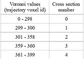
The final refinement concerns objects having multiple cross sections along a single trajectory, for example as in a subway station having floors with different lengths along the railway track. In this case, the algorithm allows for using a library of cross sections (Fig. 13). In the example presented we have three different ones, and an additional two to mark the boundaries between those by placing a vertical wall perpendicular to the trajectory. A lookup table (Table 1) on the Voronoi image is used to select amongst the models in the library (Fig 14).
Whereas in the previous example the reader might consider it doubtful to be presented a subway station with a sharp bend in the middle, this final example shows a smooth curve. This possibility, however, was already covered by the algorithm of Section 3.
Table 1: Lookup table indicating different cross section image depending on the locations along the trajectory
Voronoi values (trajectory voxel id)
Cross section number
0 - 298 0
299 - 300 1
301 - 358 2
359 - 360 3
361 - 399 4
In all the above cases it is required to slightly smoothen the Voronoi image, in order to ensure its continuity (within the discretization limitations).
Fig. 14: Model consisting of multiple cross sections
5. CONCLUSION
We have presented an algorithm for reconstruction of elongated objects with fixed cross sections, extending along arbitrary trajectories. Both input and output of the algorithms are structured as rasters, in 2d and 3d respectively. The process greatly benefits from an output driven approach, which ensures that the correct value is once and only once assigned to each voxel in the resulting 3d model, without requiring any post processing.
We also presented extensions of the algorithm to handle sloped trajectories, perpendicular cut-offs and models using multiple cross sections, each of these on the basis of the Voronoi image, which comes as a by-product of distance transform. We expect the algorithm to be a useful extension of a toolbox, which we have under construction in the course of an effort to map underground infrastructure in urban environments, and to integrate it with above-ground voxel models (Gorte and Zlatanova, 2016).
References
Arya S., D. M. Mount, N. S. Netanyahu, R. Silverman and A. Wu, 1998, Optimal Algorithm for Approximate Nearest Neighbor Searching in Fixed Dimensions, Journal of the ACM, 1998, 45(6): pp. 891-923
Birken R., D. E. Miller, M. Burns, P. Albats, R. Casadonte, R. Deming, T. Derubeis, Th. B. Hansen, M. Oristaglio, 2002. Efficient large-scale underground utility mapping in New York city using a multichannel ground-penetrating imaging radar system. Proc. SPIE 4758, Ninth International Conference on Ground Penetrating Radar, 186 (April 15, 2002); doi:10.1117/12.462307
Borgefors G., 1989, Distance transformations in digital images, Computer Vision, Graphics, and Image Processing Volume 34, Issue 3, pp. 344-371
Eisemann, E. and Décoret, X., 2008, Single-pass GPU solid voxelization for real-time applications, Proceedings of Graphics Interface 2008, pp. 73-80
Foley J.D., A. van Dam, S.K. Feiner and J.D. Hughes, 1996, Computer Graphics Principles and Practice, Addison-Wesley, 1996.
Gorte B. and W Koolhoven, 1990, Interpolation between isolines based on the Borgefors distance transform, ITC Journal 1990 No. 3, pp. 245-249
Gorte, B, and S. Zlatanova, 2016, Rasterization and voxelization of two- and three-dimensional space partitionings. Int. Arch. Photogramm. Remote Sens. Spatial Inf. Sci., 2016, XLI-B4, pp. 283-288
Konecny, G, 2003, Geoinformation: Remote Sensing, Photogram-metry and Geographical Information Systems, Taylor and Francis
Nooruddin F. and G. Turk, 2003, Simplification and Repair of Polygonal Models Using Volumetric Techniques, IEEE Trans. on Visualization and Computer Graphics, vol. 9, nr. 2, April 2003, pp. 191-205
Serra J., 1988, Image Analysis and Mathematical Morphology, Volume 2: Theoretical Advances, Academic Press, ISBN 0-12-637241-1