The social cost of labor in rural development:
job creation benefits re-examined
Theodore M. Horbulyk
∗Department of Economics, University of Calgary, Calgary, Alta., Canada T2N 1N4
Received 19 November 1998; received in revised form 24 October 1999; accepted 24 February 2000
Abstract
Job creation effects are examined as they would apply to social analysis of rural development programming by public or private sector agencies. A synthesis and critique are provided of approaches to valuing the social opportunity cost of labor. These approaches vary according to whether or not unemployment is present in the pre-project state and according to whether or not there is interregional migration in response to project hiring. Graphical, partial equilibrium analysis illustrates why, in general, job creation and project employment give rise to social costs, not benefits. The magnitude of these social costs is shown to depend upon the presence of payroll taxes, wage subsidies and unemployment, in addition to the market’s supply and demand elasticities. These social costs may be reduced or offset in specific instances where projects increase the value of labor’s productivity or reduce its costs, such as with job training, worker mobility and skill development projects. Careful attention to these approaches can help society choose correctly among alternative development proposals and among alternative (labor-intensive versus capital-intensive) technologies. © 2001 Elsevier Science B.V. All rights reserved.
JEL classification:D6; J3; O2; Q1
Keywords:Social opportunity cost; Labor; Cost-benefit analysis
1. Introduction
Governments in developed and developing coun-tries are attempting to implement policies that favor rural economic growth and simultaneously reduce existing unemployment or underemployment of labor. By reference to recent published examples, this pa-per shows that some analysis has not paid sufficient attention to the social cost of labor employed when job creation is pursued in the private or public sector. In specific instances, policy analysis has confused the socialcostof labor with the distributionalbenefitthat
∗Tel.:+1-403-220-4604; fax:+1-403-282-5262. E-mail address:[email protected] (T.M. Horbulyk).
is potentially achieved through job creation. Correct analysis is important both in choosing among alter-native development proposals and in choosing among alternative (labor-intensive versus capital-intensive) technologies. The paper illustrates these issues using static, partial equilibrium analysis of labor market ad-justment, with and without regional migration. When correctly conceptualized, the social costs and benefits of job creation policies can best inform a range of rural policy decisions.
The next section of this paper outlines a number of concepts used to assess the costs and benefits to soci-ety from employing a specific class of labor in either the public or private sector such as part of some ru-ral development project or job creation scheme. The
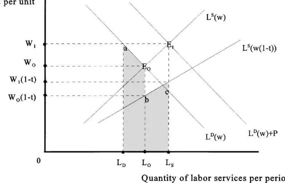
Fig. 1. Labor market adjustment without involuntary unemployment.
following section expands those concepts to labor mar-kets that incorporate interregional migration as an ad-justment process. These concepts are then applied to re-examine, conceptually, the appropriate assignment of social opportunity costs and job creation benefits in rural development applications.
The principal contribution of this paper is to provide a clear synthesis of these economic welfare concepts as they relate to labor use in rural development program-ming, and to highlight by reference to published coun-terexamples, the need to apply them assiduously.1
2. Concepts in labor cost measurement
Fig. 1 will be used to identify and distinguish a number of important concepts in labor cost measure-ment. Fig. 1 illustrates a market for a specific class of labor services both before and after a rightward shift in the demand curve, where the demand curve shifts due to increased employment associated with a rural development project or a job creation scheme. Fig. 1
1Much of the analytical framework that is presented here is
a synthesis of arguments originally presented by Little and Mir-rlees (1969), Harberger (1969), Harris and Todaro (1970), Mishan (1971), Dasgupta et al. (1972) and Heckman (1974). Boadway and Bruce (1984) review many of these approaches, but they do not provide comparative diagrammatic analysis nor do they ad-dress the alternative conceptual approaches that give rise to the potential (and actual) confusion that remains in the literature.
is drawn under the assumptions that (i) there is one freely operating labor market without any influence from interregional migration, and (ii) this market does not experience significant unemployment or underem-ployment at the initial market wage level.2
The demand for labor ex ante is portrayed by the curve LD(w), a derived demand based on the social value of the marginal product labor. This assumes away other positive or negative externalities due to employment or due to the production technology. Let
Pindicate the quantity of labor services hired by the project per period. When the demand curve shifts (to
LD(w)+P) the entire increase in demand is directly at-tributable to the project under the assumption that ex-isting private labor demands will not also increase. (In other words, this is deterministic, comparative static, partial equilibrium analysis of labor market behavior. The analysis excludes significant income effects in this and other markets due to the project.) The labor sup-ply curve,LS(w), is indicative of the social marginal cost of individuals’ labor supply decisions, and
incor-2 The labor market may exhibit a significant unemployment rate
porates the social valuation of individuals’ utility of leisure foregone and disutility of labor in this type of employment. By assumption, there are no other posi-tive or negaposi-tive externalities due to employment.
In Fig. 1 there is an existing distortionary ad val-orem tax at rateton wages,w. In equilibrium atE0,
the tax causes a misallocation of labor relative to a ‘first-best’ outcome. AtE0the marginal social benefit of the last unit employed, w0, exceeds the marginal
social cost,w0(1−t), by the amount of the tax. Since
this tax is the only source of labor market distortion (by prior assumption) the tax causes the labor sup-ply curve (drawn as a function of the pre-tax market wage,LS(w)), to lie everywhere to the left of the so-cial marginal cost (SMC) of labor curve,LS(w(1−t)). By convention in what follows, market wages,w, are reported on a before-tax basis as in the initial equilib-rium atE0. The equilibrium after-tax wage,w0(1−t),
can be illustrated either by the height of the curve
LS(w(1−t)) atL0, or by the height of an alternate
la-bor demand curve,LD(w(1−t)) atL0, where the latter
curve is not shown here or in the subsequent analysis.3 In general, the market’s adjustment to new hiring due to the project will put upward pressure on market wages and increase the observed (equilibrium) level of employment toLS atE1. The quantity of labor ser-vices hired by the project per period,P, appears as the horizontal distance, (LS−LD), between the original
and new labor demand curves. There are two distinct sources of the P units of new labor services sup-plied to the market: some are displaced or ‘crowded out’ from other employers, (L0−LD), and the others,
(LS−L0) are new entrants to the labor market. Each
source of labor can be costed separately.
Following the approach of Harberger (1969, 1971) the labor that is displaced from other employers causes a decrease in their output and the social cost of this
la-3Taxes are employed as a pre-existing ‘generic’ distortion in
the analysis that follows. The present analysis generalizes to cases where the rate of tax,t, is positive, zero or negative. If zero, taxes can be ignored and the curvesLS(w) andLS(w(1−t)) coincide.
If the tax rate is positive, the tax might instead be levied at a fixed rate per hour, in which case the two supply curves would be drawn in parallel. If the tax rate were negative, this would signify the presence of distortionary labor subsidies. If a labor subsidy value were greater than (less than) other labor taxes, the social marginal cost of labor curve would be everywhere to the left of (to the right of) the labor supply curve that is a function of the subsidized or taxed wage rate.
bor should be valued at the social marginal value prod-uct of labor for these (L0−LD) units. This is shown as
the left shaded area in Fig. 1, with unit values of US$ w0tow1dollars per hour, the tax inclusive wage. The
labor that is provided by new entrants should be valued at its social marginal cost per unit for these (LS−L0)
units. This is shown as the right shaded area in Fig. 1, with values of US$w0(1−t) to w1(1−t) dollars per
hour, the after-tax wage. Since these labor services are provided after the wage increase but not before, this (range of) wage(s) represents these suppliers’ ‘reserva-tion wage’ — the least amount each supplier is willing to accept to offer his or her labor services to the market. One could estimate a shadow wage rate (i.e. a social opportunity cost per unit of labor) that was a weighted average of the before-tax and after-tax wages, where the weights would depend on the rel-ative shares of each source of new labor supply. For instance, if one kneww0 andt, and if one could
es-timate the own-price elasticities of labor supply and demand atE0, then one would have a ready basis for
estimating this weighted average using established formulae (Harberger, 1969).4 This estimate would represent the opportunity cost per unit of project la-bor to society, where the terms ‘society’ and ‘social’ apply to a well defined reference group (e.g., the pop-ulation of a region, state or country) on whose behalf the project or policy decision is being evaluated.
There are grounds for confusion about the opportu-nity costs that society incurs in undertaking this project hiring, and this confusion may revolve around some of the other measures of market value also represented in Fig. 1. For example, one observes that (w1×P) will
be the per period payroll expenditure of the project, which amount is, in general, neither a measure of so-cial cost nor soso-cial benefit. Indeed, in this example,
4 In the case where either the supply curve or the demand curve
were infinitely elastic or inelastic, the weights would reduce to zero and unity such that eitherworw(1−t) would represent the social opportunity cost of labor (Harberger, 1969). Furthermore, with infinitely elastic demand or supply, the valueswandw(1−t), respectively, would be precise measures of unit costs, whereas for zero and other elasticity values, this approach would provide approximations to the true values. Where distortionary taxes or subsidies are levied at significant rates in labor markets, the ap-propriate choice of before-tax or after-tax wage values can be the critical step in defining the correct social opportunity cost, even where the observed wage change due to the project (w1−w0) is
payroll expenditure (as a financial cost to a project) exceeds the social opportunity cost of labor expendi-ture — the area (w1×P) exceeds the shaded areas in
Fig. 1. Part of this expenditure is a transfer of surplus to labor and part of it is a transfer of tax revenues to the public treasury.
There are alternative ways to derive the exact same shaded areas in Fig. 1 as the relevant measure of social opportunity cost from project hiring actions. Recall that these shaded areas denote the change in social welfare, monetized here as changes in Marshallian consumers’ surplus (and reported in US dollars per period, for example).5 One alternative approach is to recognize that these shaded areas are precisely the ag-gregation of all gains and losses to specific subgroups in society: workers, employers, the project funders, and the public treasury. Under the present assump-tions, these are the only social subgroups who incur costs or benefits due to these labor market transactions. The workers gain an increase in their surplus (eco-nomic rents) since wages have increased and exceed transfer earnings for all but the last unit employed. Employers in the market lose surplus on two accounts: they pay more per hour for those units of labor they retain and they lose workers for whom they were pre-viously earning ‘consumers’surplus’. The project ex-pends a material sum on the payroll each period, which in a narrow sense, is a cost to the project. Finally, the treasury gains (payroll) tax revenues which form a benefit once they become available for other uses. If one carefully identifies each of these amounts on Fig. 1 and subtracts those that are losses from those that are gains, the result is precisely the shaded areas shown previously, representing a per-period cost to society.6
5Compensated measures of welfare change, such as equivalent
variation and compensating variation, can be defined by reference to areas under a compensated labor supply curve, for example, and would not necessarily yield the same monetary measures.
6In Fig. 1, the project payroll expenditure (w
1×P=w1×
(LS−LD), shown by area:LDaE1LS,) and loss of consumers’
sur-plus (area: w1aE0w0) appear as negative entries and are
off-set by the gain in surplus to labor (area: w0(1−t)bcw1(1−t))
and the (unambiguous) increase in wage tax revenues ((w1×t×LS)−(w0×t×L0)). The net effect is a negative per period
flow equivalent in area toLDaE0bcLS, the shaded areas in Fig. 1.
As in the general literature on shadow pricing, there might also be related social costs or benefits associated with increases or de-creases in the level of distortions in related markets, such as those for substitute or complementary factors.
3. The cost of labor in a market with involuntary unemployment
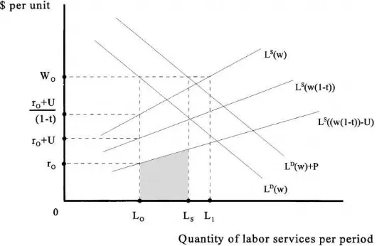
Consider now the relaxation of the full employment assumption made earlier. If there is involuntary unem-ployment that exists prior to the project, then the evalu-ation of social cost needs to be expanded to include this market characteristic. Fig. 2 illustrates this situation for some market other than that shown in Fig. 1. At the market wage,w0, the quantity of labor supplied,L1,
exceeds the quantity of labor demanded,L0, defining involuntary unemployment of (L1−L0) units of these labor services per period. It is important to note that this situation would be counterfactual to that illustrated in Fig. 1 and that the labor supply behavior described in Fig. 2 does not coexist with that illustrated earlier. For example, the pre-project employment level,L0, in
Fig. 1 exhibits a reservation wage ofw0(1−t) and the
market is in equilibrium, whereas in Fig. 2 the reserva-tion wage is lower and the market isnotin equilibrium. Indeed, in the general case of involuntary unemploy-ment, one cannot observe the level of the reservation wage before or after the project, and its estimation may require the use of non-market valuation techniques.
In Fig. 2, the project’s use of labor shifts the market demand curve to the right by the horizontal distance
P, but not far enough to employL1, the quantity of labor supplied atw0. There is no upward pressure on
market wages due to the project and no crowding out of labor services from other employers. Some quantity of labor services (LS−L0) becomes employed and the
cost that society incurs thereby will be the reservation wage associated with these units. As before, this social cost will incorporate individuals’ valuations of leisure (or of household production activities) foregone and of disutility of labor in this type of employment and will rarely be zero.
An added wrinkle to the evaluation of this situation, is that involuntarily unemployed individuals may be in receipt of some form of unemployment insurance or targeted transfer payments (in cash or in kind) for which the individuals become ineligible once they ac-cept employment. Suppose these payments are equal in value to US dollars per hour. Letr0be the
(unob-servable) reservation wage as before, the least dollar amount the marginal labor supplier is willing to accept to offer his or her services to the market. Then (r0+U)
Fig. 2. Labor market adjustment with involuntary unemployment.
accept, and ((r0+U)/(1−t)) is the smallest before-tax
wage they would accept, and these values are used as labels for the height of the various labor supply curves atL0in Fig. 2. Note that each of the three labor
sup-ply curves is a representation of the same individuals’ labor supply behavior expressed in explicitly different units of measure.
If one is able to determine that involuntary un-employment exists prior to the project but cannot observe r0, there may still be a basis for estimating
the range within which r0 must fall. The existence
of involuntary unemployment at L0 implies thatw0
is strictly greater than ((r0+U)/(1−t)). Together with
the previous assumptions, this implies that the net market wage (w0(1−t)−U) exceedsr0, which, in turn,
presumably exceeds zero. This provides numerical bounds (0≤r0<(w0(1−t)−U)) on the unobservable
value,r0, where the value of the upper bound should
be readily observable from the existing market data. Thus, where involuntarily unemployed workers are drawn into the market by a project, the social marginal cost of employing the first of them will be r0, and for allP of them will be the dollar value per period represented by the shaded area in Fig. 2. Unlike the areas in Fig. 1, the specific area in Fig. 2 cannot be estimated directly from market data collected prior to the project. Fortunately, available market data will support a range of estimates within which the actual value will lie. Non-market valuation techniques, such as contingent valuation could be used to refine one’s
estimate, although one should first determine whether project outcomes are in fact sensitive to these estimates prior to dedicating costly analytical resources.
As before, one can distinguish that project em-ployment gives rise to financial expenditures (w0×P)
that may exceed the social opportunity cost by a con-siderable margin. This employment may also reduce unemployment transfers and may increase (wage) tax receipts.There will also be a gain in surplus to labor where a worker’s net wage (after-tax and forego-ing unemployment transfers) exceeds the reservation wage for all but the last unit hired. It is essential to keep in mind that these other values are simply alternative ways of deriving the shaded cost area al-ready shown in Fig. 2, and are not extra sources of cost or value that can be added in.7 As will be seen presently, much confusion remains in the literature on precisely these points.
In practice, a project’s employment of labor may draw on the involuntarily unemployed, as well as on the voluntarily unemployed and on workers hired away from other employers. In these cases the social
7 Specifically the social opportunity cost shown by the shaded
area in Fig. 2 can be constructed (precisely) by starting with the financial expenditures (w0×(LS−L0)) as a cost to
employ-ers, and allowing as offsetting benefits: (i) the reduction in unemployment transfers (U×(LS−L0)); (ii) the increased tax
receipts ((w0×t)×(LS−L0)); and (iii) the gain in surplus to labor
((w0(1−t)−U)×(LS−L0)) minus each labor unit’s reservation
opportunity cost per hour will be a weighted average of the opportunity costs identified for each of the three sources individually.
4. Labor costs in the presence of interregional migration
Sometimes one also needs to relax the assumption that there is a single labor market within which ad-justments occur without interregional migration. In these instances, there is a small number of other fac-tors that one needs to introduce to one’s estimation of the social costs of labor. Specifically, the social cost of quantities of labor supplied to the market in which the project hires must incorporate three cost elements that will be in addition to those covered in Figs. 1 and 2. These are the costs incurred in the region from which the labor originates; the migration costs incurred, and the possibility that some multiple of in-dividuals migrates for each employment position that is created. Each of these three social cost elements will be described briefly.
When the net effect of project hiring in one region is that some number of workers is hired away from another region — whether hired now by the project di-rectly or by other employers in the new project region — then one must turn attention to the labor-exporting region to assess a social opportunity cost for each unit of labor that migrates. Equilibrium market wage lev-els may differ across regions due to non-monetary dif-ferences in the characteristics of the regions or of the jobs, due to mobility barriers, or due to other types of market segmentation. Analysis of social costs must look beyond market wage levels to determine the na-ture of the market adjustments that will occur in the labor-exporting region. Generally this analysis will involve determining how much labor is drawn away from alternative employment (incurring a social cost in output foregone) and how much is provided from among the ranks of the voluntarily or involuntarily un-employed (at a social cost based on their respective reservation wages).
For those labor services that are provided by work-ers who have migrated, there may be additional social costs associated with the migration decision. These migration costs may be financial, such as the in-creased costs of living in the importing region, or they may be non-financial, such as the extra dollar
amount one would expect to receive in order to locate (voluntarily) away from family, friends, and familiar or preferred surroundings and the compensation one would expect in return for extra risks borne. These (social) migration costs may be time-limited or con-tinuing depending on their nature. All are relevant costs that, conceptually, society should capture or include on a dollar basis when estimating the social costs of the new jobs that are filled.
It is well known from the work of Harris and Todaro (1970) that labor markets may be segmented (or dual-istic) such as by institutional or legal barriers and that this can support differing equilibrium market wage levels. In this class of labor markets, interregional mi-gration can be the source of adjustment when a rural development project creates jobs in one region. Al-though the specific numerical estimates will depend on such factors as the risk preferences of the migrants and the migration flows that result, an expected out-come is that the rate of labor migration toward the area with project hiring may exceed the rate of hir-ing itself, and this migration may increase the rate of unemployment or underemployment in the receiving region. If there is reason to suspect that these adjust-ment processes are active, then a proper estimate of the social cost of employment must be based on an es-timate of the total costs incurred — not only by those hired, but by the larger set of individuals induced to migrate (Jenkins and Kuo, 1979; Boadway and Bruce, 1984, pp. 302–306).
Table 1 provides data and a brief example of how the social opportunity cost per unit of project labor could be estimated using the approaches illustrated by Figs. 1 and 2. To motivate the calculation, consider a road construction project typical of those underway in rural areas of Nepal. Typically, an intense annual program of construction activity in the dry season can make use of seasonally underemployed agricultural labor for unskilled construction tasks. International donors provide considerable funding and might ask that cost benefit analysis be undertaken, such as to pri-oritize this work. The project would use some skilled labor, overseers and machinery, not shown in Table 1, and these costs would be estimated separately as part of a larger project evaluation exercise.
Table 1
Estimation of the social opportunity cost of unskilled labor for a road building project, based on the sources of labor used and applying the methods of Figs. 1 and 2a
Market source of unskilled labor services expected to be procured for project
Basis for estimating social opportunity cost (SOCL)
Social opportunity cost per week in domestic currency (NRs)
Percentage of total labor expected to come from each market source (%)
Fraction of SOCLby
source (column 3×column 4) (NRs/week)
Same district
Previously employed w0 380 10 38.0
Voluntarily unemployed w0(1−t) 323 10 32.3
Involuntarily unemployed r0 200 40 80.0
Neighboring district
Previously employed wˆ0+m 360 5 18.0
Voluntarily unemployed wˆ0(1−t )+m 315 5 15.8
Involuntarily unemployed r0+m 260 30 78.0
Total 100 SOCL=262.1
aThe tax rate ist=0.15. The value of unemployment benefit per period isU=0. The wage rate in the neighboring district,wˆ 0= ˆw1=
300, which is less than in the project district wherew0=w1=380, which is also the uniform project wage paid for unskilled labor. There
is an ongoing migration cost borne by each migrant,m=60, and all migrants find employment. The reservation wage,r0=r1=200, is same
in each district.
estimates of the portion of this project labor force that will come from the project locale (60%), and the por-tion (40%) that will bear some personal cost (m) to migrate to the project district from neighboring dis-tricts. The composition of each of these two labor pools is described, further, in terms of those who are drawn away from other employment, and those who drawn from voluntary or involuntary unemployment. For simplicity, the project life here is one season. In a multiyear project, the relative prices of labor and the composition of the labor pools might be projected to change over the project life, and this would be re-flected in each year’s expenditures.
On the assumption that the road project does not induce excessive migration from other districts (e.g. no encampments of prospective project job seekers are expected) the social opportunity cost per unit of unskilled project labor becomes a weighted average of the costs of workers from each of six sources. The bottom line shows that project labor represents a social cost, albeit a social cost that is only about 70% of the actual project wage rate,w0.
5. A re-examination of costs and benefits
The labor market concepts and labor cost defini-tions described so far were developed and refined over a number of years, yet they have not been well
assimilated nor appreciated by the economics, agri-cultural economics and rural development policy pro-fessions in general. As a result, there are numerous and continuing examples in the academic literature and in the practice of project evaluation that do a disservice to their audiences by misrepresenting the appropriate social costs of project labor use. This section will address selected general issues that per-sist and then cite some examples of a more specific nature.
The first point to be reinforced by all of the forego-ing is that the profession does its greatest service by emphasizing and re-emphasizing that, first and fore-most, job creation and employment creation give rise to social costs not benefits. These are the costs iden-tified by the shaded areas in Figs. 1 and 2. Although in a market with taxes or unemployment, for example, these employment costs may be smaller in magnitude than the project’s payroll expenditures, they are costs all the same. Of course, a project will ideally generate social benefits too, but these are best assessed in rela-tion to goods and services produced, not in relarela-tion to factor inputs used. If extra goods and services could be produced without any use of labor, project benefits would result all the same.
benefits must be identified and assessed on their spe-cific merits. For example, in many markets, there will be projects that undertake labor education, job train-ing and skill development. These projects can increase the social value of the marginal product of labor (or decrease its marginal social cost), and these increases may be temporary or permanent. Such gains may be intended to spill over to non-project employers. There might be positive net returns from investment in labor market institutions such as investments that reduce the (equilibrium) rates of structural and frictional unemployment, or that reduce inequity in the work-place. Some programs might supply labor to a market with a specific skill shortage shifting the supply curve rightward (instead of shifting the demand curve as in the figures above). However, this sub-class of rural development projects is but one small part of the rural development investment portfolio, and the labor these projects employ still gives rise to a social opportunity cost to accompany these valid and identifiable labor market benefits.
A third point is that the assessment of social costs and benefits is a markedly different exercise than the identification and measurement of social or (macro-) economic impacts. Although project decision mak-ers will also be interested in impacts, it is important to acknowledge that, whereas larger payrolls almost certainly increase a project’s economic impacts, these larger payrolls may or may not increase project net benefits.8
By decomposing, for each of Figs. 1 and 2, the ag-gregate social cost into separate elements that benefit or harm specific social sub-groups such as employ-ers, workemploy-ers, project funders and the public treasury, the foregoing analysis makes clear that there may be an important distributional benefit associated with
8In the world of unpublished project evaluation reports, it is
common to observe authors’ confusion over the relevance of eco-nomic impacts to project or policy selection decisions. This author is aware of one example where the project consultants decided that project employment expenditure had a multipliedimpacton the regional economy, and that this impact must surely be seen as a benefit to the project region. By extension, therefore, all other operating expenditures were categorized as benefits. Thus, the con-sultants summed all labor and operating expenses and entered a multiple of them on the benefit side of their benefit-cost ledger with no further consideration of labor as a social cost. The er-ror in their analysis was the failure to distinguish between social impactsand socialbenefits.
project employment. Obviously, workers will gain surplus from increased employment, so that from this sub-group’s perspective, job creation will appear as a benefit and not a cost. Moreover, project employment may create a specific benefit to society as a whole if it provides a lower cost method of redistributing income or wealth than other available alternatives — such as where effective tax and transfer systems do not exist — and if society places a sufficiently high value on this redistribution.
The analysis of labor market behavior described in the figures and tables does not address the so-called ‘indirect effects’ of labor and other factor use, de-fined to be those which occur in markets other than those where the project transactions are occurring. For example, using more labor may cause increased en-vironmental degradation, increased traffic congestion and so on, where these costs to society will be rel-evant to social project evaluation and decision mak-ing. Similarly, there may be associated social gains and losses when the project decreases or increases the amounts of public funds that need to be raised (at some social cost) by the public treasury. A com-prehensive analysis of project costs and benefits will include the net social costs of all such indirect ef-fects, in addition to evaluating — as in Figs. 1 and 2 — those costs and benefits which occur directly in the markets where the project procures inputs or sells outputs.
If errors are made in the field by lay practitioners, it is perhaps less excusable to have them ordained by the procedural manuals produced by central funding agencies.9 Consider the case of the federal govern-ment of Australia whose Handbook of Cost-Benefit Analysis (1991) was written as a resource document and guide for public servants and others, especially for evaluating and appraising projects with major resource implications. When it comes to address the issue of involuntary unemployment (as this paper illus-trates in Fig. 2) the Handbook provides the following advice:
“. . .Provided that there is a significant gap between the level of unemployment benefits and the pre-vailing net of tax wage, one can reasonably infer that some workers would be willing to accept a
9 See Belli et al. (1996) for an example of recent
take-home wage that is below the net of tax wage rather than remain unemployed. Provided people place a positive value on leisure or their involve-ment in unpaid work, it is inappropriate to assume that there is a zero opportunity cost in employing labor which would otherwise be unemployed. At a minimum, therefore, the shadow price of labor is likely to equal the value of unemployment bene-fits plus some amount in compensation of foregone leisure.” (Australia, Department of Finance, 1991, p. 34)
In the notation of Fig. 2, the Handbook is rec-ommending that the shadow price of labor (i.e. its social opportunity cost per unit) be assumed to lie in a range above (U+r0) where U would represent
the unemployment benefits and r0 would represent
compensation to the individual for leisure foregone. This contradicts the advice given here which is to use the reservation wage, r0, as the social
opportu-nity cost at the margin, full stop. The advice here is to choose a value for the unobservable r0 in the
range between zero and (w0(1−t)−U) where this
en-tire range may exclude the value recommended by the Handbook for some values of the variables w0, r, t
andU.
The Handbook, in essence, treats every dollar of unemployment transfers foregone by new workers as a social cost, whereas the present advice, for the reasons accompanying Fig. 2, says no part of them is a cost — with the following intuition. The individual receives an hourly amountUeither as part of the transfer if the individual foregoes project employment and pursues leisure, or as part of a higher wage if the individual foregoes leisure and pursues the job. The amount U
becomes irrelevant to the individual’s choice and is thereby irrelevant to social cost since the amount is received independent of whether labor services are provided to the project or not.10 The amountUis not
10The marginal social cost of capital associated with raising the
public funds used to pay the amounts U (such as by taxation or borrowing), could also be introduced to the analysis. These foregone financing charges would give rise to a social benefit when payments of U are reduced through project employment. Conversely, the Australian Handbook (1991) seeks to treat foregone unemployment benefits as a social cost. Correctly stated, the value of reduced unemployment transfers would enter social analysis as a social benefit, equal in value to the foregone social costs of financing these transfer payments.
part of the worker’s (or society’s) opportunity cost. Only the extra dollar amount (above and beyondU) compensates the individual for leisure foregone, and that amount alone will form a relevant indicator of the reservation wage.11
Perhaps little would be served by cataloguing ex-tensively the many instances where the social benefits and costs of job creation have been misrepresented by analysts working in this area, other than to highlight the continuing need for greater attention to these is-sues. After all, according to Little and Mirrlees (1991, p. 360) as recently as 1990 the economic appraisal of projects for The World Bank did not even systemat-ically estimate or use shadow wage rates. However, following an economist’s variant of the Hippocratic oath, if such values are to be employed, at least one should do no harm.
References
Australia, Department of Finance, 1991. Handbook of Cost-Benefit Analysis. Australian Government Publishing Service, Canberra.
Belli, P., Anderson, J., Barnum, H., Dixon, J., Tan, J.P., 1996. Handbook on Economic Analysis of Investment Operations. The World Bank, Washington.
Boadway, R.W., Bruce, N., 1984. Welfare Economics. Basil Blackwell, Oxford.
Dasgupta, P., Sen, A.K., Marglin, S.A., 1972. Guidelines for Project Evaluation. United Nations Industrial Development Organisation, New York.
Drèze, J., Stern, N., 1987. The theory of cost-benefit analysis. In: Auerbach, A.J., Feldstein, M. (Eds.), Handbook of Public Economics, Vol. 2. North-Holland, Amsterdam, pp. 909–989.
Harberger, A.C., 1969. Discussion: Professor Arrow on the social discount rate. In: Somers, G.G., Wood, W.D. (Eds.), Proceedings of a North American Conference on Cost-Benefit Analysis of Manpower Policies. Kingston, Canada, Queen’s University, Industrial Relations Centre, pp. 76–88.
Harberger, A.C., 1971. On measuring the social opportunity cost of labor. Int. Labor Rev. 103, 559–579.
Harris, J.R., Todaro, M.P., 1970. Migration, unemployment and development: a two-sector analysis. Am. Econ. Rev. 60, 126– 142.
Heckman, J., 1974. Shadow prices, market wages and labor supply. Econometrica 42 (4), 679–694.
11Dr`eze and Stern (1987, pp. 964–967) formalize these points,
Jenkins, G., Kuo, C.-Y., 1979. On measuring the social opportunity cost of permanent and temporary employment. Can. J. Econ. 11 (2), 220–239.
Little, I.M.D., Mirrlees, J.A., 1969. Manual of Industrial Project Analysis in Developing Countries, Vols. I and II. Organisation for Economic Cooperation and Development, Development Centre, Paris.
Little, I.M.D., Mirrlees, J.A., 1991. Project appraisal and planning twenty years on. In: Fischer, S., de Tray, D., Shah, S. (Eds.), Proceedings of the World Bank Annual Conference on Development Economics 1990. The World Bank, Washington, pp. 351–382.