CLOUD REMOVAL FROM SENTINEL-2 IMAGE TIME SERIES THROUGH SPARSE
RECONSTRUCTION FROM RANDOM SAMPLES
D. Cerra∗, J. Bieniarz, R. M¨uller, P. Reinartz
German Aerospace Center (DLR), Earth Observation Center (EOC), 82234 Weling, Germany (daniele.cerra, jakub.bieniarz, rupert.mueller, peter.reinartz)@dlr.de
Commission III, WG III/3
KEY WORDS:Sentinel-2, Clouds, Image Time Series, Image processing, Pre-processing.
ABSTRACT:
In this paper we propose a cloud removal algorithm for scenes within a Sentinel-2 satellite image time series based on synthetisation of the affected areas via sparse reconstruction. For this purpose, a clouds and clouds shadow mask must be given. With respect to previous works, the process has an increased automation degree. Several dictionaries, on the basis of which the data are reconstructed, are selected randomly from cloud-free areas around the cloud, and for each pixel the dictionary yielding the smallest reconstruction error in non-corrupted images is chosen for the restoration. The values below a cloudy area are therefore estimated by observing the spectral evolution in time of the non-corrupted pixels around it. The proposed restoration algorithm is fast and efficient, requires minimal supervision and yield results with low overall radiometric and spectral distortions.
1. INTRODUCTION
Satellite Image Time Series (SITS) are sets of images acquired by the same or different spaceborne sensors over the same area at multiple acquisition times. In recent years, both the availabil-ity and the temporal resolution of SITS acquired by multispectral sensors is increasing steadily. An important challenge for the fu-ture is the processing of SITS acquired by the Sentinel-2 mission, which will make available multispectral SITS at global scale with a frequent revisit time of less than 5 days, once both satellites of the constellation will be in orbit (Drusch et al., 2012). It would be desirable then to identify algorithms requiring limited supervi-sion and computational resources to improve the automated pro-cessing chain of these datasets.
One hindrance for the analysis of SITS acquired by optical sen-sors is the presence of thick clouds in the scenes within a multi-temporal stack, which makes difficult to observe the evolution of a given ground cover in time. In recent years, researchers have found sparse reconstruction techniques to outperform traditional methods based on based on temporal replacement or patch-based spatial replacement (Shen et al., 2015).
Recently, Sparse Unmixing-based Denoising (SUBD) has been successfully applied for the inpainting of missing values in op-tical earth observation data. SUBD estimates the value of cor-rupted pixels based on their sparse decomposition in terms of un-corrupted image elements, making only an indirect use of spatial information. In the case of scenes affected by thick clouds within a SITS, an effective restoration is usually possible if information about the missing image elements is given in cloud-free acquisi-tions in the multitemporal stack. A large set of cloud-free pixels can be selected to model the evolution in time of the ground cov-ers in a given scene, as sparse methods excel at handling what are known as overcomplete dictionaries, i.e. a set of training samples which can be much larger than the dimensionality of a dataset, which for a multispectral SITS is proportional to the number of spectral bands per image and to the number of temporal acquisi-tions.
∗Corresponding author
The efficiency and automation of SUBD can increase when the atoms in the overcomplete dictionary used for the reconstruction are randomly selected from the image, as selecting a large number of elements in the dictionary increases the performance minimis-ing the reconstruction error yielded by a given dictionary. This allows providing results in quasi real-time. Furthermore, the se-lection of a random dictionary implies that dictionary sese-lection, usually requiring several parameters to set and computational re-sources when carried out by explicitly avoiding coherent entries or minimising reconstruction errors, only requires the setting of the number of elements to be extracted. This can be chosen ac-cording to the size of the analysed images and the number of cloud-free acquisitions available for a given stack. Another ad-vantage of working with sparse methods is their efficiency, as it is possible to use specialized algorithms and data structures ex-ploiting the sparse nature of the handled data, requiring limited computational resources with respect to methods which operate on dense matrix structures.
This paper presents the first results of applying SUBD for sparse reconstruction of missing information in multitemporal Sentinel-2 datasets, based on non-corrupted samples randomly acquired from the same images. A mask for clouds and clouds shadows must be given, and it is manually derived in our case. Given the difficulties in the future to process the large amount of Sentinel-2 multitemporal data stacks that will be available, this paper also moves towards an automation of the method, indicating how to set adaptive thresholds in order to process these datasets in an unsupervised way.
The paper is structured as follows. Section 2 gives a reminder on the sparse reconstruction techniques adopted by the algorithm. Section 3 reports the first experimental results of the method ap-plied to a Sentinel-2 data stack. We conclude in Section 4.
2. SPARSE UNMIXING-BASED DENOISING (SUBD)
Unmixing-based Denoising (UBD), an algorithm which in its orig-inal conception restored bands affected by a low Signal-to-Noise Ratio (SNR) in hyperspectral images (Cerra et al., 2014). Hy-perspectral datasets feature a high number of narrow, adjacent spectral bands often in the order of hundreds, while as a com-parison typical multispectral sensors have less than 10 (broader) bands and Sentinel-2 has 13 bands at different spatial resolutions (Drusch et al., 2012).
UBD is based on the concept of spectral unmixing, which aims at decomposing each hyperspectral image element into a linear (or less often non-linear) combination of signals representing the backscattered solar radiation in each spectral band from a target within the image or analysed in laboratory. The considered tar-gets are typically composed of a single pure material or a homo-geneous mixture of materials, and are often called endmembers (Bioucas-Dias et al., 2012): in this paper we simply refer to them as reference spectra in order to adopt a consistent nomenclature. The output of a spectral unmixing process is a set of abundances maps, quantifying the contribution of each reference spectrum to a given pixel. In a linear spectral mixture a pixelmcould be expressed as:
thek available and pre-selected reference spectra, whiler is a residual vector containing the portion of the signal which cannot be represented in terms of the basis vectors of choice.
The output of the spectral unmixing process in eq. 1 is then in-ferred into UBD’s reconstruction process. By considering the physical properties of a mixed spectrum, the residual vectorr is assumed to be mostly composed by noise and more relevant in spectral bands where atmospheric absorption effects are stronger, and therefore ignored in the reconstruction.
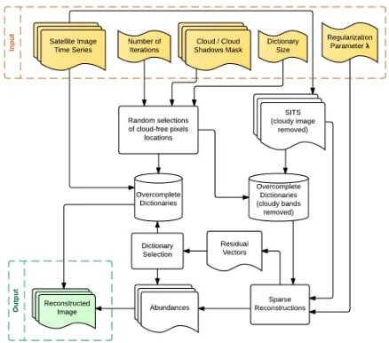
Figure 1. Workflow for the described method. In orange the re-quired input (data and parameters), in green the output. Most of the required input parameters can be empirically or adaptively derived without requiring too much supervision.
Better results have been obtained by coupling UBD with sparse reconstruction techniques (Cerra et al., 2015). In sparsity-based
spectral unmixing, most of the abundances xi in Equation (1) are equal to zero, as these methods assume that only a few ref-erence spectra contribute tom, and the abundance vector to be estimated is therefore sparse. The use of sparse unmixing within the UBD workflow resulted in the definition of Sparse Unmixing-based Denoising (SUBD), which can be carried out as follows.
In the first step a spectral dictionaryAis derived by collecting a large number of image elements, randomly selected from the area which is cloud-free in all the images in the stack. The dictionary is overcomplete, meaning that the number of entries it contains is higher than the dimensionality of the data. The use of overcom-plete libraries for sparse reconstruction have been widely used in the past; see, for example, (Iordache et al., 2011), (Bieniarz et al., 2015), and (Tang et al., 2014). Afterwards, each image element yand the dictionaryAare fed to a non-negative version of the least angle regression LASSO (LARS/LASSO) reconstruction al-gorithm (Efron et al., 2004), which guarantees a sparse solution by solving the following minimization problem:
minx|Aˇx−yˇ|22 s.t. |xˇ1| ≤λ,xˇ≥0 (2)
whereyˇis the original image from which the corrupted bands have been removed, andxˇcontains the fractional abundances for the spectra selected in the reconstruction ofyˇ, without consider-ing the bands belongconsider-ing to the corrupted image. The regulariza-tion parameterλis the upper bound on theℓ1norm controlling
the sparsity of the solution vector ˇx. The regularization prob-lem in eq. 2 is especially advantageous when the dictionaryA is overcomplete: this is the case for the large spectral libraries used in SUBD, which are also highly coherent (Bioucas-Dias et al., 2012, Bieniarz et al., 2015). This motivates the choice of the LARS solver, which is robust in dealing with dictionaries having the mentioned characteristics (Bach et al., 2011).
It is important to remark that in the problemxˇmust be used in-stead ofx, as including in the dictionaries the values of corrupted bands (covered by clouds) would introduce relevant error in the abundance estimation step. Instead, the reconstruction is esti-mated in the cloud-free portion of the stack. To give an informal example, consider a pixelp1 below a cloud in the first image of
a stack containingnacquisitions, and that in the rest of the stack the spectro-temporal patternp2...nis composed by50%ofD1 and50%ofD2, whereDiis theithentry in a dictionary. If in
eq. 2 the bands fromp1would be included in the dictionary, the
real abundance values could be reconstructed with relevant errors. Instead, the pixelp1 can be reliably reconstructed as a subset of
p= 0.5D1+ 0.5D2, as the relative dictionary entries have been
collected from areas of the image which are cloud-free also in the corrupted portion of the stack.
With respect to previous works, instead of selecting the median value for each reconstruction after running the process several times, in this paper we select separately the best dictionary for each pixel, chosen in order to yield the minimum value forrafter the reconstruction in eq. 1. This increases the probability that all type of materials or ground covers below the cloud can be cor-rectly reconstructed if they are present also outside of the clouds and selected in any of the dictionaries, as this would yield the minimum reconstruction error.
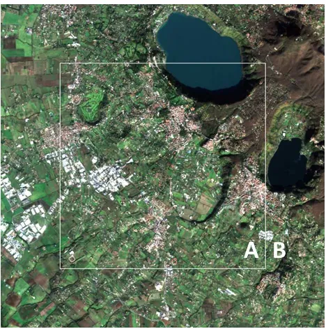
Figure 2. True color combination for a cloud-free subset from the Sentinel-2 Stack analysed in this paper. The area denoted with an A is assumed to be covered by thick clouds and therefore invisible. The dictionaries used for the sparse reconstruction are built by collecting random pixels from the area in a buffer around the cloud, denoted with a B.
the setting of theλregularization parameter, a value of 1 usu-ally yields satisfactory results whenever the dictionary entries are collected from the same image (Cerra et al., 2016). With the dic-tionary size empirically set as will be detailed in next Section, the only parameter requiring further investigations is the number of iterations. From preliminary analysis, results did not change significantly after 50 iterations, so we set this specific parameter to 50 in the reported experiments.
3. EXPERIMENTAL RESULTS
We analyse a stack of four images acquired over an area close to the city of Rome, Italy, in a timespan ranging from the 18th of December 2015 to the 17th of January 2016. A550×550 sub-set which is cloud-free in all the images is selected, and only the bands with a spatial resolution of 10 or 20 meters are kept for a to-tal of 10 spectral bands per image. The three bands with a spatial resolution of 60 meters are discarded, and the bands at higher res-olution are resampled to 20 meters after applying a Gaussian filter separately to each one to prevent aliasing. Please note that this is done only to simplify the workflow: the bands could be kept at their original resolution by applying the method separately to the three groups of spectral bands, with no degradations in perfor-mance (Cerra et al., 2016).
After the subset is selected, occlusion by a cloud of size350×350 is simulated in the center of the image (area A in Fig. 2). A to-tal of 50 dictionaries D is built by collecting for each of those 20 random spectra from the stack in the area outside of the cloud, de-noted by a B in Fig. 2. The number of elements|D|for each dic-tionaryDis chosen applying the empirical rule defined in (Cerra et al., 2016):
|D|= min{5N,100} (3)
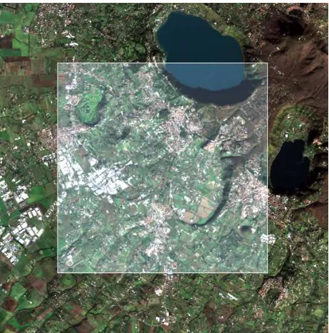
Figure 3. True color combination for the restoration of the area denoted with an A in Fig. 2.
In whichNis the dimensionality of the subspace containing the relevant information in the dataset. To estimateNmethods tradi-tionally applied to hyperspectral image processing could be used (Bioucas-Dias and Nascimento, 2008). In this case we applied a Principal Component (PC) transform to the Sentinel SITS and select a number of dimensions which contains more than 98.5% of the total variance of the dataset. For the described stack, these conditions are met by selecting the first four PCs after the rota-tion, soNis set to 4 and|D|to 20.
Afterwards, SUBD as described in eq. 2 is applied, and the image is reconstructed according to the dictionary yielding the smallest residual vector for each pixel. Results are reported in Fig. 3. The images are visually very similar, with smooth transitions on the borders between the reconstructed obscured pixels and the cloud-free ones. Results are assessed quantitatively by estimating the absolute reconstruction error and spectral distortion across the 10 considered bands in the affected image. For the former, the figure of merit is the Mean Average Error (MAE) across all the considered 10 spectral bands expressed in percentage, while the latter is quantified through the mean Spectral Angle (SA) (Kruse and al., 1993). Results are reported in Table 1.
MAE SA
1.08% 4.5×10⁻²
Table 1. Mean Average Error (MAE) and Spectral Angle (SA) for the cloud removal experiment in the area denoted by an A in Figs. 2 and 3.
of that field, this can be reliably reconstructed. On the other hand, local changes on the field below the cloud such as specific crop marks cannot be restored.
Results could be provided to the end users simply as restored images, or by overlaying a transparent white layer on the recon-structed areas, in order to clearly show which pixels have been synthesized and are therefore less reliable than the ones which were cloud-free in the first place. An example for this visualiza-tion is reported in Fig. 4.
4. CONCLUSIONS
This paper presents the first results of applying Sparse Unmixing-based Denosing (SUBD) to cloud removal in single scenes of Sentinel-2 SITS. Pixels covered by clouds are restored through sparse reconstruction, with the employed dictionaries composed of randomly selected cloud-free pixels.
To increase the automation of the method, a set of dictionary composed by randomly selected image elements is considered, and for the restoration of each pixel the dictionary yielding the minimum reconstruction error in the available cloud-free bands is selected. This allows selecting with high probability a given dic-tionary which contains the spectro-temporal patterns of the ma-terials of which the pixel of interest is composed. These will be more than one if the image element to be reconstructed is mixed, thing which is likely at Sentinel-2 ground sampling distances. First results on a data stack acquired close to the city of Rome in Italy are satisfactory both objectively and subjectively, as they are visually very similar to the test image and are restored with low reconstruction errors.
The method is not suitable for cases in which information on the contaminated pixels is corrupted but available, as in the case of haze, as it completely ignores the cloudy pixels in the reconstruc-tion process. For this purpose, algorithm coming from the field of atmospheric correction should be employed instead.
In the future, traditional methods based on substitution of the con-taminated pixels with cloud-covered ones will be integrated in the workflow. The reconstruction process will resort to these alterna-tive algorithms whenever the residual vector is too high, indicat-ing that probably the materials composindicat-ing a given pixel below the cloud have not been found in any dictionary extracted from the cloud-free areas around the sensitive one. Another improve-ment would be represented by a better characterization of the area from which the dictionaries are extracted, increasing the proba-bility that a selected dictionary entry contains a material which is also present to some degree in the area below the cloud. If the cloud mask is available, a possible choice would be creating a buffer around the cloud, and forcing the dictionary entries to be selected from the area defined by the buffer: this would go in the direction of the experiments in Section 3 for the simulated square cloud therein.
REFERENCES
Bach, F., Jenatton, R., Mairal, J., Obozinski, G. et al., 2011. Con-vex optimization with sparsity-inducing norms.Optimization for Machine Learningpp. 19–53.
Bieniarz, J., Aguilera, E., Zhu, X. X., M¨uller, R. and Reinartz, P., 2015. Joint sparsity model for multilook hyperspectral image unmixing. Geoscience and Remote Sensing Letters, IEEE12(4), pp. 696–700.
Figure 4. Alternative visualization option for an end user, in which a transparent cloud is simulated and overlaid to visually distinguish original image elements from synthesized ones.
Bioucas-Dias, J. and Nascimento, J., 2008. Hyperspectral sub-space identification. IEEE Transactions on Geoscience and Re-mote Sensing46(8), pp. 2435 –2445.
Bioucas-Dias, J. M., Plaza, A., Dobigeon, N., Parente, M., Du, Q., Gader, P. and Chanussot, J., 2012. Hyperspectral unmixing overview: Geometrical, statistical, and sparse regression-based approaches. IEEE Journal of Selected Topics in Applied Earth Observations and Remote Sensing5(2), pp. 354–379.
Cerra, D., Bieniarz, J., Beyer, F., Tian, J., M¨uller, R., Jarmer, T. and Reinartz, P., 2016. Cloud removal in image time series through sparse reconstruction from random measurements.IEEE Journal of Selected Topics in Applied Earth Observations and Remote Sensing.
Cerra, D., Bieniarz, J., M¨uller, R., Storch, T. and Reinartz, P., 2015. Restoration of simulated enmap data through sparse spec-tral unmixing.Remote Sensing7(10), pp. 13190.
Cerra, D., M¨uller, R. and Reinartz, P., 2014. Noise reduction in hyperspectral images through spectral unmixing. IEEE Geo-science and Remote Sensing Letters11(1), pp. 109–113.
Drusch, M., Del Bello, U., Carlier, S., Colin, O., Fernandez, V., Gascon, F., Hoersch, B., Isola, C., Laberinti, P., Martimort, P. et al., 2012. Sentinel-2: Esa’s optical high-resolution mission for gmes operational services. Remote Sensing of Environment120, pp. 25–36.
Efron, B., Hastie, T., Johnstone, I. and Tibshirani, R., 2004. Least angle regression.Annals of statistics32(2), pp. 407–499.
Iordache, D. M., Bioucas-Dias, J. and Plaza, A., 2011. Sparse unmixing of hyperspectral data.Geoscience and Remote Sensing, IEEE Transactions on49(6), pp. 2014–2039.
Kruse, F. and al., 1993. The Spectral Image Processing System (SIPS) - Interactive Visualization and Analysis of Imaging Spec-trometer Data.Remote Sensing of Environment44, pp. 145–163.
data: A technical review. Geoscience and Remote Sensing Mag-azine, IEEE3(3), pp. 61–85.