STATISTICS FOR PATCH OBSERVATIONS
K. L. Hingeea,b∗
aCSIRO, Underwood Ave, Floreat, Perth, Australia
bSchool of Mathematics & Statistics, University of Western Australia, Stirling Highway, Perth, Australia
Youth Forum
KEY WORDS:random closed sets, landscape pattern indices, land cover, thematic maps, spatial statistics
ABSTRACT:
In the application of remote sensing it is common to investigate processes that generate patches of material. This is especially true when using categorical land cover or land use maps. Here we view some existing tools, landscape pattern indices (LPI), as non-parametric estimators of random closed sets (RACS). This RACS framework enables LPIs to be studied rigorously. A RACS is any random process that generates a closed set, which encompasses any processes that result in binary (two-class) land cover maps. RACS theory, and methods in the underlying field of stochastic geometry, are particularly well suited to high-resolution remote sensing where objects extend across tens of pixels, and the shapes and orientations of patches are symptomatic of underlying processes. For some LPI this field already contains variance information and border correction techniques. After introducing RACS theory we discuss the core area LPI in detail. It is closely related to the spherical contact distribution leading to conditional variants, a new version of contagion, variance information and multiple border-corrected estimators. We demonstrate some of these findings on high resolution tree canopy data.
1. INTRODUCTION
Statistical analysis of images can be grouped into two main branches (Molchanov, 1997): (a) describing/classifying an observed scene or (b) considering the scene to be gener-ated by a random process and inferring properties of this process. We are concerned mostly with the latter, and es-pecially those processes observed in remotely sensed maps of categorical variables. Such analysis occurs when com-paring different regions, comcom-paring the same region at dif-ferent times, gaining understanding of random processes (e.g. spatial dependence), or model fitting.
A random closed set (RACS) is a generic framework for modelling randomness in processes that generate spatial patterns of patches. It encompasses common models in re-mote sensing, such as those derived from Markov random fields and Gaussian random fields, and a wide range of other models (e.g. germ-grain models, birth-growth mod-els, fibre processes, and tessellations). Markov random fields excel at contextual investigations, but have diffi-culty describing geometrical properties (Descombes, 2012). Gaussian random fields, completely determined by their mean and covariance (Chiu et al., 2013), can only capture first and second order characteristics of a process. Other RACS models can describe complex geometrical shapes and infinite-order characteristics (Descombes, 2012). These models reveal new methods for describing the geometry of random scenes such as contact distributions (Baddeley and Gill, 1994) and tangent point analysis (Barbour and Schmidt, 2001).
These tools have been combined with remote sensing to model uncertain object boundaries (Zhao et al., 2009), me-teorological features (Cressie et al., 2012), fine-scale grass
∗Corresponding author
patterns (Sadler, 2006) and urban tree locations (Rossi et al., 2015). The RACS framework has also been used to test the spatial dependence of beetle infestation (Kautz et al., 2011) and the relationship between tree deaths and bore locations (Chang et al., 2013). Numerous other examples exist (Descombes, 2012).
We examine parallels between non-parametric RACS sum-mary functions and landscape pattern indices (LPI). To the author’s knowledge this is the first published discus-sion on this topic. A RACS framework leads to more rig-orous treatment of landscape pattern data and improved understanding of LPI behaviour, including border correc-tions, resolution robustness and conditional probabilities. In the next section we introduce RACS theory in more detail, with a focus on concepts relevant to remote sens-ing applications. Subsequently Section 3 discusses RACS and LPI. Finally Section 4 describes an application of non-parametric RACS estimators to maps of tree canopy.
2. RANDOM CLOSED SETS AND REMOTE SENSING
For brevity we omit many technical details and the full generality of RACS. These details can be found in a num-ber of texts (Molchanov, 2005; Chiu et al., 2013). A RACS is any random process that generates a closed set. Aclosed
set in Euclidean space is any set for which all points on the edge of the set are also in the set. A RACS, X, is then any process that maps from some state space Ω to closed subsets of Euclidean space
P(X(ω)is closed) = 1. (1)
produces categorical maps if its realisations are closed 2D regions. This definition allows only two classes, insideX
or not insideX, but can be generalised to multiclass real-isations (Molchanov, 1984; Ayala and Sim´o, 1995; Kautz et al., 2011).
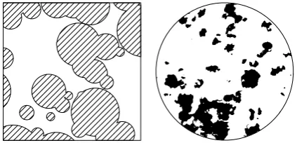
Figure 1: Example realisations of RACS.Left: A Boolean model (Stoyan and Mecke, 2005) observed in a rectangular region; hatched regions denote locations inside the random
set. Right: A map of tree canopy which can be represented
as a realisation of a RACS. This is also an example of the observations used in Section 4.
As an example the pattern of mould on the surface of an old slice of bread can be modelled as a RACS. The mould pattern may have some systematic properties (e.g. patch size) but the precise location, size and shape of the mould is unpredictable. For this RACS a single realisation is the pattern of mould on a single slice of bread.
The mathematical field underlying the statistical investi-gation of random scenes is known as Stochastic Geometry (Molchanov, 1997). It is the study of statistical meth-ods for geometrical patterns (Matheron, 1975; Chiu et al., 2013). Historically an important application has been the inference of 2D or 3D properties (e.g. properties of rocks) from lower dimensional samples (Baddeley and Jensen, 2004). This application area, known as stereology, has developed tools for inference from 0D samples (e.g. pixels) and from images (2D samples).
Often it is the case in remote sensing of the Earth that only one realisation of the process is available. For ex-ample the generation of a native forest, including all its past disturbances, is usually seen only once at each lo-cation. We can mitigate this issue by assuming that the statistical properties of the process are similar at different locations and that the dependence between distant loca-tions is small. Thus observaloca-tions of different regions act like multiple realisations. These sort of assumptions are common in spatial analysis.
The strongest similarity assumption isstationarity which assumes the statistical properties of a process are transla-tion invariant. In other words the probability of any closed, bounded setKintersectingX, writtenP(K∩X 6=∅), is independent of translations ofK; the probability depends only on the shape and size ofK. As an example consider the centre of the mouldy bread slice at high magnification so that we may ignore the border of the bread and assume that the process is stationary. This stationarity assump-tion implies that, before looking at the bread, the prob-ability that any particular location is mouldy P(x∈X), known as the coverage probability, is the same for all x. It also means that the probability that a circular region contains mould depends only on the radius, which leads to
the spherical contact distribution (SCD) discussed later.
These examples correspond to intersecting with a set{x}
and a disc respectively. The stationary assumption has been common in landscape ecology (Fortin et al., 2003).
There are a number of summary functions that are well de-fined for stationary RACS. A summary function describes particular properties of a RACS, typically as a probabil-ity or the expectation of some quantprobabil-ity. Examples are the coverage probability, the spherical contact distribution and the expected perimeter-length per unit area. They have been used to fit parameters and uniquely determine pa-rameters for some model classes (Hug et al., 2002).
Once we have observed something about the mould, near locationasay, then the conditional probability of an event nearb,P(event nearb|event neara), is not usually trans-lation invariant because it depends on the location of b
relative to a. In general RACS observations at different locations can be very dependent.
A stationary process is mixing if, as b gets further away froma, the probability,P(event nearb|event neara), ap-proaches the value that it would have assuming indepen-dence. Stationary and mixing processes areergodic(Daley and Vere-Jones, 2008,§12.3) which means spatial averages of large windows may be used instead of averages across multiple realisations. For example if the bread mould pro-cess is ergodic then the probability of a particular loca-tion being mouldy can be estimated by the proporloca-tion of mouldy locations in a large window; multiple slices of bread are not needed. Note that in practice the stationarity as-sumption requires observations in windows small enough that changes in the environment (e.g. a distant change in soil type) can be ignored whilst estimates using the er-godic property require large windows. The window size is then a compromise between estimator accuracy and the credibility of the stationarity assumption.
3. AN APPLICATION TO LANDSCAPE PATTERN INDICES
Landscape ecologists study both the effect of spatial pat-tern on ecological processes wherein spatial patpat-tern is con-sidered a covariate and the effect of ecological processes on spatial pattern wherein the spatial pattern is considered a response or symptom of the ecological process (Fortin and Agrawal, 2005). Frequently this requires comparing pat-terns observed in remotely sensed maps of land cover type.
LPIs are numerical descriptions of spatial configuration that are commonly used in landscape ecology (Lustig et al., 2015). Current LPIs have proved sensitive to resolu-tion and boundary effects (Kupfer, 2012). Many LPIs are also difficult to interpret (Schr¨oder and Seppelt, 2006) and highly correlated with other LPIs (Cushman et al., 2008; Schindler et al., 2008; Turner, 2005). There have been numerous calls for more rigorous statistical interpretation of LPIs (Lustig et al., 2015; Dramstad, 2009; Wang and Cumming, 2011) and some calls for more process-based metrics (Fortin et al., 2003; Remmel and Csillag, 2003). RACS provide a generic probabilistic framework that al-lows statistical interpretation, process-based descriptions and rigorous study of LPI behaviour.
from FRAGSTATS (VanDerWal et al., 2015). Within the collection of metrics available in FRAGSTATS we have noticed that:
1. The percentage of landscape index is an estimator of coverage probability
2. The edge density index is a (potentially biased) esti-mator of an identically named concept in RACS the-ory.
3. The percentage of core area is an estimator of thecore
probability which is related to the spherical contact
distribution for a RACS.
4. The description of the radius of gyration given by (Keitt et al., 1997) is related to the mean star of in-tersection of a RACS (Molchanov, 1997).
5. Variants of the contagion index can be constructed that express second-order and geometric properties of RACS.
A crucial contribution here is that LPIs can be viewed as estimators of underlying random processes. To the author’s knowledge this is the first time non-parametric RACS summary functions have been explicitly correlated with LPI concepts. Kautz et al. (Kautz et al., 2011) pro-vide an example of the power of non-parametric RACS very similar to LPI without directly referring to LPIs. Oth-erwise previous use of RACS in relation to LPIs have been for simulation studies (Hargis et al., 1998) and model fit-ting (Diggle, 1981; Sadler, 2006).
The remainder of this section discusses the core area, the closely related SCD, and a new contagion index that uses the SCD. The new SCD-based contagion is less resolu-tion dependent than the classic pixel-adjacency contagion. For core area, the RACS perspective provides variance in-formation, border corrections and natural conditioning on events. We will also make use of the coverage probability which is easily estimated by the percentage of landscape. The details for other indices will be discussed in a forth-coming paper.
In the following suppose that X is a stationary, mixing RACS process, and that we have observed a single realisa-tion,Xobs, in a windowW.
3.1 Percentage of Core Area
For a user chosen buffer distance,r, core area is the area within a class that is more thanr distance from the edge of the class (McGarigal, 2015; Didham and Ewers, 2012). The percentage of core area in a window is an estimate of the probability that a point will be further thanrdistance from the exterior of X. This is also the probability of placing a disc of radiusrentirely withinX,
Percentage of core area≈P(Br(o)⊆X), (2)
whereBr(o) is a disc of radiusrabout the origin,o. The
origin is used here arbitrarily because the stationarity ofX
requires that the probability is the same regardless of the disc’s centre. Thus the analogous concept of core area for a random process could be described as Core Probability
and is the probability that a point will be further thanr
distance from the exterior ofX. In the next section (Sec-tion 3.1.1) we show that core probability is closely related to the SCD.
3.1.1 Core Probability and the SCD. The SCD (also known as theempty space function) is a popular tool for exploration and inference of random point processes (Baddeley et al., 2015) and sets (Diggle, 1981; Molchanov, 1997; Heinrich, 1993). The unconditional version is the probability ofX intersecting an arbitrarily located disc of radiusr,
SCDXunc(r) =P(Br(o)∩X 6=∅). (3)
where∅is the empty set so ‘6=∅’ can be read as ‘not empty’ and we have arbitrarily used the origin as the centre of the disc.
The conditional version of the SCD is the probability ofX
intersecting a disc given that the centre of the disc is not inX,
SCDcond
X (r) =P(Br(o)∩X6=∅|o /∈X). (4)
Ifo∈X thenX intersects the disc so the two versions are related by
where pis the coverage probability. Recall that the cov-erage probability is the probability of an arbitrary point being inX, it can be estimated by the percentage of W
covered byXobs(Baddeley and Jensen, 2004).
The SCD describes the sizes of space outsideX; a RACS with a large conditional SCD at radius r is less likely to contain gaps in which a disc of radiusr can fit.
The space that is not interior to X is also a RACS, we denote it by Xc. The superscript ‘c’ denotes the set of
locations not inXand the overline represents the inclusion of the edges. IfX is stationary then so isXcand thus the
SCD ofXcis well defined. Furthermore the unconditional
SCD of Xc is the probability that an arbitrarily located
disc of radiusr intersectsXc which is the negation of the
core probability. In other words
SCDunc
The conditional version is the probability that a point in
X is within distancerof the outside ofX
SCDcondXc (r) =P(Br(o)∩Xc6=∅|o /∈Xc) (7)
which suggests a conditional core probability (CCP), the probability that a point inX is in the core ofX,
conditional core probability = 1−SCDXcondc (r)
=P(Br(0)⊆X|o∈X).
(8)
Thus the non-parametric properties of the unconditional and conditional SCD are identical to those of the core prob-ability and the CCP respectively.
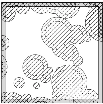
3.1.2 Border Correction. Estimation of the core probability using percentage of core area risks making an implicit assumption aboutX outside the observation win-dow. See Figure 2. There are points which appear further thanr distance from the edge ofXobsbut may not be in
larger with larger buffer distance because the area within
r distance of the boundary is a larger proportion of the window area. We mention three different border corrected estimators for the unconditional SCD that are available in the spatstat package within the R statistical computing en-vironment (Baddeley et al., 2015). For brevity we describe them only in terms of the core probability. Despite the-oretical differences the three estimators perform similarly well in simulation experiments for a variety of random pat-terns of points (Stoyan, 2006; Baddeley et al., 2015), which suggests that they will also perform with similar quality on RACS. Note that the CCP can be estimated from the ratio of a core probability estimate and a coverage probability estimate.
The reduced sample estimate uses only those points further than r distance from the window’s boundary (Heinrich, 1993). See Figure 2. Due to the different sample size for each r the estimated core probability can increase as the buffer distance increases, however an increase in the true core probability is not possible because a point not in the core of X for buffer distancer cannot be in the core for larger buffer distances.
The Chiu-Stoyan correction uses the length of the set of points exactlyk distance from the boundary ofXobsand
integrates k between 0 and the desired radiusr. It pro-duces estimates for each radius r that are unbiased and can not increase with r, but there is a chance that the estimate will pass below 0 (Chiu and Stoyan, 1998).
Alternatively the Kaplan-Meier correction, which uses methods for the analysis of censored survival times (Badde-ley and Gill, 1994), also provides non-increasing estimates of the core probability.
3.1.3 Variance. For each radius,r, the reduced sam-ple estimator is similar to the coverage probability estima-tor. Molchanov (Molchanov, 1997, §4.3) provides a vari-ance if certain properties of the process are knowna priori. It may also be possible to estimate the variance using spec-tral density (Mase, 1982; B¨ohm et al., 2004), however this method requires a suitable choice of smoothing bandwidth.
3.2 Disc-State Contagion
Contagion is a popular entropy-inspired LPI for describing aggregation of classes. The unnormalised version is defined as (O’Neill et al., 1988; Li and Reynolds, 1993)
Contagion :=
m
X
i=1
m
X
j=1
Pijln(Pij), (9)
wheremis the number of classes andPijis the probability
of randomly selected adjacent pixels being in classiand classj respectively. Although it was initially designed for multiple categories we restrict our focus to two-class maps.
Contagion as it is defined above describes the aggrega-tion of classes within a distance of double the ground sam-ple distance (double the ground samsam-ple distance because pixels are typically an average or weighted integral of the corresponding sample region). Contagions calculated at different resolutions thus describe aggregation at differ-ent scales making contagion very sensitive to resolution changes. Moreover because the definition depends on the resolution of an observation technique there is no canonical
Figure 2: An example observation of a RACS, Xobs
(hatched regions), showing points withinrdistance of the window boundary (grey region) and points that are further thanr distance from the outside ofXobs(dashed
bound-ary). The crosshatched regions are within r distance of the edge ofW and further thanrdistance from the visible edge of Xobs. Without more information it is impossible
to know whether these points are in the core area of X.
Reduced sample Estimator: The reduced sample estimator
for the core probability is the proportion of the non-grey region that is inside the dashed boundary. Chiu-Stoyan
Estimator: The Chiu-Stoyan estimator uses the length of
the dashed boundary outside the grey region given by mul-tiple smaller buffer distances to estimate the core proba-bility at the desired buffer distance.
definition for the contagion of a real landscape. A number of other metrics that use the same pixel adjacency concept have similar issues.
Ramezani and Holm (Ramezani and Holm, 2011) encoun-tered this issue when they tried to apply contagion to polygonal data. Instead they considered the adjacency probabilitiesPij to be the probability of classj
intersect-ing a circle of radius r around a point in class i. Thus contagion became a functional metric (a function of the radiusr).
We present another variant of contagion that describes the mixing of classes within a disc, termed disc-state conta-gion. Let 1 denote insideX and 0 denote outsideX. We define P10(r) as the probability that a point is in X and not in the core ofX,
P10(r) =P(o∈X, Br(o)*X), (10)
andP01(r) as the probability that a point is inXcand not in the core ofXc,
P01(r) =P(o∈Xc, Br(o)*Xc). (11)
We define the remaining elements,P11(r) as the core prob-ability ofX,
P11(r) :=P(Br(o)⊆X), (12)
and similarlyP00 as the core probability ofXc.
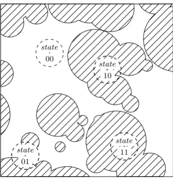
disorder of a system with four states (1) the entire disc is inX, (2) the entire disc is outsideX, (3) the centre is within X and some of the disc is outsideX, and (4) the centre is outside X and some of the disc is inside X. A diagram of each state is in Figure 3. The lowest contagion (and highest entropy) occurs when the probability of each of these states is 1
4.
This disc-state contagion can be estimated using estimates of the SCD and core probability. It is well defined for any stationary RACS, and because the disc size is not linked to resolution it is more robust to resolution changes than the classic pixel-adjacency contagion (9).
. state
00
. state
11.
. state
01
.
. state
10
.
Figure 3: Examples of each disc state in disc-state conta-gion. Hatched regions denote locations inside the realisa-tion ofX.
4. EXPLORATION OF TREE CANOPY PATTERN PROCESSES AND FEED
QUALITY
We explored decimetre resolution maps of tree canopy in Perth, Australia, using conditional SCD, CCP, disc-state contagion and coverage probability. The canopy height maps were derived from stereo photography through height estimates (stereo matching) and spectral values (Caccetta et al., 2015). Two-class categorical maps were then ob-tained by only keeping canopy that was higher than 4m.
We compared the RACS estimators with field-based anal-ysis of feed quality of Banskia woodlands for an endan-gered bird (van Dongen et al., 2016). For each location of the field-based assessment we used a circular window of 30m radius to estimate RACS properties. We randomly selected 50% of these field-assessed locations for initial ex-ploration, reserving the remaining 50% for validation.
In making these estimates it was assumed that each win-dow observed a stationary and mixing tree canopy process. Given little information on covariates such as soil, mois-ture and wind this is a tolerable representation for a first analysis.
The best gradation of feed quality was obtained by the CCP. A small cluster of very high feed quality processes appeared at core buffer distances of 0.75mand above (Fig-ure 4). In comparison the coverage probability could not
separate very high feed locations from moderate feed lo-cations (Figure 5). The SCD and disc-state contagion did not show any obvious association to feed quality (Figure 6).
Unfortunately the above discrimination of high feed loca-tions did not generalise to the validation data (Figure 7). Further exploration of other RACS summary functions and different canopy heights might uncover real associations. Discrimination might also be achieved through multi-type RACS (with each class corresponding to a different height range), 3D stochastic models, or non-stationary RACS.
Conditional Core Probability and Feed Quality
Radius (m)
Probability of being in Core
0.0 0.5 1.0 1.5 2.0
0.0
0.2
0.4
0.6
0.8
1.0
340
430
520
610
700
F
eed Quality
Figure 4: Conditional core probability for tree canopy above 4m. Each location/observation is a different curve. The colours correspond to feed quality (see colour bar on right). The canopy processes with the three highest feed quality scores (in red) are clustered together for buffer dis-tances from 0.75mto 2m(black polygon). Reduced sample boundary correction was used here but the effect was mi-nor at these distances (see Section 4.1 and Figure 8). Note that the steps in the functions were due to the map reso-lution of 0.2m, and the slight upward directions of some of these jumps was caused by the reduced sample correction.
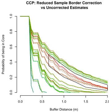
4.1 Effect of Border Correction
Border correction had little impact on the above relation-ship because the buffer distances involved were small (2m) compared to the window diameter (60m) (Figure 8). How-ever the impact of border correction on the SCD (Figure 9) suggests that CCP estimates would have been signifi-cantly impacted if the canopy patches were much larger (e.g. tens of metres in diameter).
5. COMPUTATION
Computations were performed inside the R statistical en-vironment (R Core Team, 2016) on a 3.10GHz CPU with 4GB of RAM. The spatstat package (Baddeley et al., 2015) was used heavily with tools for reading remotely sensed data provided by the raster package (Hijmans, 2015) andGDAL(GDAL Development Team, 2015). An R package containing additional necessary functions is avail-able from the author.
●
400 450 500 550 600 650 700
0.0
0.1
0.2
0.3
0.4
Coverage Probability and Feed Quality
Feed Quality
Co
v
er
age Probability
Figure 5: Coverage probability of canopy above 4mand feed quality. Each point is a different location. Note that high coverage probability suggests higher feed value, but coverage probability doesn’t discriminate between high feed locations and moderate feed locations.
1500 by 1500 pixels (300mby 300m) performing the same estimations required less than 10 seconds.
6. CONCLUSION
RACS provide a powerful generic framework for modelling the processes underlying categorical maps. They are es-pecially useful at high resolutions where the geometries created by patches of many pixels are important. The RACS framework provides a conceptual tool to guide LPI use and design including the treatment of sensing artefacts such as resolution and map extent. Here we focused on non-parametric RACS tools under the assumptions of sta-tionarity and mixing. These tools are stochastic, process-centric versions, of LPI and we discussed the core area LPI in detail.
Core area is closely related to the spherical contact distri-bution. We first linked core area to a probabilistic concept, the core probability, and then showed that core probabil-ity was the opposite of the spherical contact distribution evaluated at a particular radius. This lead to functional versions of the core probability, a conditional core proba-bility, and border corrected estimators.
The well-defined spherical contact distribution also sug-gested a resolution-free version of the contagion LPI. This new version of contagion describes the entropy of the state of a disc and its centre. The aggregation scale that this new contagion expresses is chosen by the user and is indepen-dent of the imaging resolution. In comparison the orig-inal pixel-adjacency contagion describes interaction over the width of two pixels and is thus much more sensitive to resolution change.
A preliminary exploration of tree canopy processes briefly demonstrated core probability, the spherical contact distri-bution, disc-state contagion and border corrections. Due to time restrictions the demonstrations did not include hy-pothesis tests.
Disc−State Contagion and Feed Quality
Radius (m)
Figure 6: Conditional SCD (left) and disc-state contagion (right). Curves are coloured by feed quality. There is no discernible pattern of high feed quality processes.
Conditional Core Probability
Buffer Distance (m)
Probability of being in Core
0.0 0.5 1.0 1.5 2.0
Figure 7: CCP for the validation data. The region of high feed process observed in the exploration data is shown (black polygon). The separation did not generalise to the validation data.
CCP: Reduced Sample Border Correction vs Uncorrected Estimates
Buffer Distance (m)
Probability of being in Core
0.0 0.5 1.0 1.5 2.0
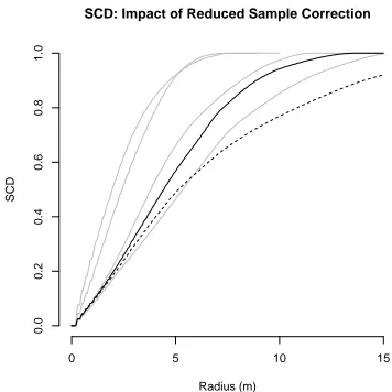
SCD: Impact of Reduced Sample Correction
Radius (m)
SCD
0 5 10 15
0.0
0.2
0.4
0.6
0.8
1.0
Figure 9: The SCD estimate for one location using re-duced sample correction (solid line) and no border cor-rection (dashed line). For context the reduced sample estimates of some other observations are shown in grey. Note that, similar to the uncorrected estimates of CCP, the uncorrected estimate of SCD is lower because it has implicitly assumed that no tree canopy existed outside the observation window. For some observations, such as the one shown here, the difference between border corrected and uncorrected estimates can be quite large. Thus using the uncorrected estimates could have serious implications for applications of the SCD.
7. ACKNOWLEDGEMENTS
Many thanks to Australia’s Commonwealth Scientific and Industrial Research Organisation for supplying the tree canopy maps, and to Ricky van Dongen and Geoff Bar-rett of Western Australia’s Dept. of Parks and Wildlife for providing the feed data.
I would also like to thank my PhD supervisors Adrian Baddeley, Peter Caccetta, and Gopalan Nair.
References
Ayala, G. and Sim´o, A., 1995. Bivariate random closed sets and nerve fibre degeneration. Advances in Applied
Probability27(2), pp. 293–305.
Baddeley, A. and Gill, R. D., 1994. The empty space haz-ard of a spatial pattern. Technical report, Department of Mathematics, University of Utrecht. Preprint 845.
Baddeley, A. and Jensen, E. B. V., 2004. Stereology for
Statisticians. Monographs on Statistics & Applied
Prob-ability, Vol. 103, Chapman and Hall/CRC, Boca Raton, Florida.
Baddeley, A., Rubak, E. and Turner, R., 2015. Spatial
Point Patterns: Methodology and Applications with R.
Chapman and Hall/CRC, London.
Barbour, A. D. and Schmidt, V., 2001. On Laslett’s trans-form for the Boolean model. Advances in Applied
Prob-ability33(1), pp. 1–5.
B¨ohm, S., Heinrich, L. and Schmidt, V., 2004. Kernel estimation of the spectral density of stationary random closed sets.Australian & New Zealand Journal of Statis-tics46(1), pp. 41–51.
Caccetta, P., Collings, S., Devereux, A., Hingee, K., Mc-Farlane, D., Traylen, A., Wu, X. and Zhou, Z., 2015. Monitoring land surface and cover in urban and peri-urban environments using digital aerial photography.
In-ternational Journal of Digital Earthpp. 1–19.
Chang, Y., Baddeley, A., Wallace, J. and Canci, M., 2013. Spatial statistical analysis of tree deaths using airborne digital imagery. International Journal of Applied Earth
Observation and Geoinformation21, pp. 418–426.
Chiu, S. N. and Stoyan, D., 1998. Estimators of distance distributions for spatial patterns. Statistica Neerlandica
52(2), pp. 239–246.
Chiu, S. N., Stoyan, D., Kendall, W. S. and Mecke, J., 2013. Stochastic Geometry and Its Applications. 3 edn, John Wiley & Sons.
Cressie, N., Assuncao, R., Holan, S., Levine, M., Nicolis, O., Zhang, J. and Zou, J., 2012. Dynamical random-set modeling of concentrated precipitation in North
Amer-ica. Statistics and its Interface5(2), pp. 169–182.
Cushman, S. A., McGarigal, K. and Neel, M. C., 2008. Parsimony in landscape metrics: Strength, universality, and consistency.Ecological Indicators8(5), pp. 691–703.
Daley, D. and Vere-Jones, D., 2008. An Introduction to the Theory of Point Processes II: General Theory and
Structure. Probability and its applications, Vol. 2, 2
edn, Springer Science, New York, N.Y., United States.
Descombes, X. (ed.), 2012. Stochastic Geometry for Image
Analysis. ISTE / John Wiley & Sons.
Didham, R. K. and Ewers, R. M., 2012. Predicting the im-pacts of edge effects in fragmented habitats: Laurance and Yensen’s core area model revisited. Biological
Con-servation155, pp. 104–110.
Diggle, P. J., 1981. Binary mosaics and the spatial pattern of heather. Biometrics37(3), pp. 531–539.
Dramstad, W. E., 2009. Spatial metrics – useful indicators for society or mainly fun tools for landscape ecologists?
Norsk Geografisk Tidsskrift - Norwegian Journal of
Ge-ography63(4), pp. 246–254.
Fortin, M. and Agrawal, A. A., 2005. Landscape ecology comes of age. Ecology86(8), pp. 1965–1966.
Fortin, M. J., Boots, B., Csillag, F. and Remmel, T. K., 2003. On the role of spatial stochastic models in un-derstanding landscape indices in ecology. Oikos102(1), pp. 203–212.
GDAL Development Team, 2015. GDAL - geospatial data abstraction library. Version 2.0.0 http://www.gdal.org (3 Mar. 2016).
Hargis, C. D., Bissonette, J. A. and David, J. L., 1998. The behavior of landscape metrics commonly used in the study of habitat fragmentation. Landscape Ecology
Heinrich, L., 1993. Asymptotic properties of minimum contrast estimators for parameters of Boolean models.
Metrika40(1), pp. 67–94.
Hijmans, R. J., 2015. raster: Geographic data anal-ysis and modeling. Version 2.5-2 http://CRAN.R-project.org/package=raster (3 Apr. 2016).
Hug, D., Last, G. and Weil, W., 2002. A survey on contact distributions. In: K. Mecke and D. Stoyan (eds),
Mor-phology of Condensed Matter, Lecture Notes in Physics,
Springer Berlin Heidelberg, pp. 317–357.
Kautz, M., D¨ull, J. and Ohser, J., 2011. Spatial depen-dence of random sets and its application to disperion of bark beetle infestation in a natural forest. Image
Anal-ysis & Stereology30(3), pp. 123–131.
Keitt, T. H., Urban, D. L. and Milne, B. T., 1997. Detect-ing critical scales in fragmented landscapes.
Conserva-tion ecology1(1), pp. 4.
Kupfer, J. A., 2012. Landscape ecology and biogeography: Rethinking landscape metrics in a post-FRAGSTATS landscape. Progress in Physical Geography 36(3), pp. 400–420.
Li, H. and Reynolds, J. F., 1993. A new contagion index to quantify spatial patterns of landscapes. Landscape
Ecology8(3), pp. 155–162.
Lustig, A., Stouffer, D. B., Roig´e, M. and Worner, S. P., 2015. Towards more predictable and consistent land-scape metrics across spatial scales.Ecological Indicators
57, pp. 11–21.
Mase, S., 1982. Asymptotic properties of stereological es-timators of volume fraction for stationary random sets.
Journal of Applied Probability19(1), pp. 111–126.
Matheron, G., 1975. Random sets and integral geometry. John Wiley & Sons, USA.
McGarigal, K., 2015. FRAGSTATS help. Tech-nical report, University of Massachusetts. http://www.umass.edu/landeco/research/fragstats/ documents/fragstats documents.html (12 May 2015).
Molchanov, I., 1984. Labelled random sets. Theory of
Probability and Mathematical Statistics29, pp. 113–119.
Molchanov, I., 1997. Statistics of the Boolean Model for
Practitioners and Mathematicians. John Wiley & Sons.
Molchanov, I. S., 2005.Theory of random sets. Probability and its applications, Springer, London.
O’Neill, R. V., Krummel, J. R., Gardner, R. H., Sugihara, G., Jackson, B., DeAngelis, D. L., Milne, B. T., Turner, M. G., Zygmunt, B., Christensen, S. W., Dale, V. H. and Graham, R. L., 1988. Indices of landscape pattern.
Landscape Ecology1(3), pp. 153–162.
R Core Team, 2016. R: A language and environment for statistical computing. Vienna, Austria www.R-project.org (3 Apr. 2016).
Ramezani, H. and Holm, S., 2011. A distance dependent contagion function for vector-based data.Environmental
and Ecological Statistics19(2), pp. 161–181.
Remmel, T. K. and Csillag, F., 2003. When are two land-scape pattern indices significantly different? Journal of
Geographical Systems5(4), pp. 331–351.
Rossi, J., Garcia, J., Roques, A. and Rousselet, J., 2015. Trees outside forests in agricultural landscapes: Spatial distribution and impact on habitat connectivity for for-est organisms. Landscape Ecology31(2), pp. 243–254.
Sadler, R., 2006. Image-based modelling of pattern dy-namics in a semiarid grassland of the Pilbara, Australia. PhD, School Of Plant Biology, University of Western Australia, Perth, Australia. (Thesis).
Schindler, S., Poirazidis, K. and Wrbka, T., 2008. To-wards a core set of landscape metrics for biodiversity assessments: A case study from Dadia National Park, Greece. Ecological Indicators8(5), pp. 502–514.
Schr¨oder, B. and Seppelt, R., 2006. Analysis of pat-tern–process interactions based on landscape mod-els—Overview, general concepts, and methodological is-sues. Ecological Modelling199(4), pp. 505–516.
Stoyan, D., 2006. On estimators of the nearest neighbour distance distribution function for stationary point pro-cesses. Metrika64(2), pp. 139–150.
Stoyan, D. and Mecke, K., 2005. The boolean model: from matheron till today. In: M. Bilodeau, F. Meyer and M. Schmitt (eds), Space, Structure and Random-ness, Lecture Notes in Statistics, Springer New York, pp. 151–181.
Turner, M. G., 2005. Landscape ecology: What is the state of the science? Annual Review of Ecology, Evolution,
and Systematics36, pp. 319–344.
van Dongen, R., Barrett, G., Zdunic, K., Huntley, B. and Mitchell, D., 2016. Food potential and night roost map-ping for calyptorhynchus latirostris using digital aerial photography. Technical report, Dept. of Parks and Wildlife, Perth, Australia. in prep.
VanDerWal, J., Falconi, L., Januchowski, S., Shoo, L. and Storlie, C., 2015. Package ‘SDMTools’: Species distribution modelling tools: Tools for pro-cessing data associated with species distribution modelling exercises. Version 1.1-221 http://cran.r-project.org/package=SDMTools (2 Apr 2016).
Wang, X. and Cumming, S. G., 2011. Measuring land-scape configuration with normalized metrics.Landscape
Ecology26(5), pp. 723–736.
Zhao, X., Stein, A. and Chen, X., 2009. Application of ran-dom sets to model uncertainties of natural entities ex-tracted from remote sensing images.Stochastic
Environ-mental Research and Risk Assessment 24(5), pp. 713–