AUTOMATIC RECONSTRUCTION OF SKELETAL STRUCTURES
FROM TLS FOREST SCENES
A. Schilling and H.-G. Maas
Technische Universität Dresden Institute of Photogrammetry and Remote Sensing
01062 Dresden, Germany [email protected]
Commission V, WG 3
KEY WORDS: Terrestrial Laser Scanning, Point Cloud Processing, Forest Inventory, Skeleton Extraction
ABSTRACT:
Detailed information about 3D forest structure is vital in forest science for analyzing the spatio-temporal development of plants as well as precise harvest forecasting in forest industry. Up to now, the majority of methods focus on complete structural reconstruction of trees from multiple scans, which might not be a suitable starting point with respect to modeling forest scenes over larger areas. For this reason, we propose a strategy to obtain skeletal structures of trees from single scans following a divide-and-conquer approach well-known from computer science. First, we split the range image into components representing surface patches and trace each component’s boundary, which is essential for our skeleton retrieval method. Therefore, we propose an extension to standard boundary tracing that takes a component’s interior depth discontinuities into account. Second, each component is processed separately: A 2D skeleton is obtained via the Voronoi Diagram and refined. Subsequently, a component is segmented into subsets of points depending on their proximity to skeleton nodes. Afterwards, the skeleton is split into paths and a Principal Curve is computed from each path’s point cluster in order to retrieve the component shape as a set of 3D polygonal lines.
Our method retrieves the intricate branching structure of components representing tree crown parts reliably and efficiently. The results are fitting with respect to a visual inspection. At present, results are fragments of tree skeletons, but it opens an attractive perspective to complete tree skeletons from skeletal parts, which we currently regard as future work.
1. INTRODUCTION
Since the turn of the century, terrestrial laser scanning (TLS) has received increasing attention as a handy tool for tasks in forestry (Hopkinson et al., 2004; Maas et al., 2008; Dassot et al., 2011). Due to international agreements about forest moni-toring and their role as a sink or source in the global carbon cy-cle, the demand for detailed information on forests has grown as well. As a result, numerous studies concentrate on the assess-ment and validation of forest inventory parameters retrieved from TLS data. Clearly, the non-destructive nature of the Li-DAR measurement principle makes laser scanning an attractive instrument to achieve long-time observation of vegetation and thus the analysis of their spatio-temporal growth that was infea-sible with conventional forestry methods in the past. But in or-der to study the spatial structure of forest ecosystems, methods that adequately reconstruct tree geometry as a compact repre-sentation have to be designed. The proposed methods can be di-vided in approaches based on voxel space analysis (Gorte and Pfeifer, 2004; Gorte, 2006; Gatziolis et al., 2010; Bucksch, 2011; Schilling et al., 2012a) and approaches that work directly on 3D point clouds (Livny et al., 2010; Raumonen et al., 2013). The retrieval of the entire tree structure is often attempted in one processing step, as for instance done by (Côté et al., 2011). However, a tree needs to be well-represented as 3D point cloud for these methods to be applicable at all. For this reason, the fo-cus of such methods has often been restricted to single, free-standing or manually isolated trees that are digitized by multiple scans. Considering the vastness of wooded areas that are of for-est-scientific interest, this kind of experimental setup poses se-rious limitations on the general applicability of the presented methods. In forest scenes, complete scan coverage of any tree simply cannot be guaranteed.
Recently, an interesting approach has been presented by (Eysn et al., 2013), who manually sketch tree skeletons in an equi-rectangular projection of TLS data. Subsequently, the skeleton sketch is used for fitting cylinders to points in the skeleton’s v i-cinity. Reconstruction is performed on single scans only. The authors point out that a step-wise reconstruction of a tree from multiple scans may be a more robust approach to a proper tree skeleton than the retrieval of the entire tree structure at once.
In this paper, we pick up the basic idea of (Eysn et al., 2013) and introduce a novel strategy to obtain skeletal structures au-tomatically from surface patches via the Voronoi Diagram and subsequent Principal Curve computation as shown in figure 1. The paper is organized as follows: First, we explain our pro-posed strategy. Subsequently, we introduce our test data and present experiment results. In section 4, we discuss open prob-lems of the presented approach. We conclude with an outlook on future work in the last section.
2. RETRIEVAL OF SKELETAL STRUCTURES
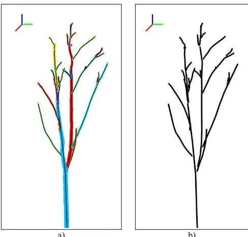
a) b)
Figure 1. Results of our strategy to retrieve spatial structure: a) Segmented 3D point cloud; colors indicate group clusters. b) Skeletal structure according to segmentation.
retrieved skeletal structures, a complete tree skeleton could be assembled in an additional processing step, which we presently regard as future work. Henceforth, we consider the term skele-ton as synonymous to skeletal structures, which both denotes the output of our method.
Our approach consists of two stages that are outlined in figure 2. In the following, the sub-procedures of our strategy are ex-plained in detail.
a)
b)
Figure 2. Two-stage processing strategy. Rounded boxes denote inputs (blue) and outputs (green). a) Segmentation of single scans into connected components. b) Retrieval of skeletal structures from components.
2.1 Preprocessing of TLS data
Commonly, output of a scan is considered to be unorganized 3D data. Although this is true for the point list exports that are used as de-facto standard output, the scanning process itself is highly ordered. As a consequence, the actual 3D data reflects this spa-tial scan pattern. (Bucksch, 2011) mentioned that this particular scan sequence is irreversibly lost if multiple scans are co-registered. Furthermore it is commonly assumed that it cannot
be recovered from TLS software directly. Therefore, it is usual-ly re-computed from the spherical coordinates. But we found that the arrangement of the TLS data in a grid-like fashion simi-lar to the intensity image is provided via the PTX format, which is often available as export option, e.g. in Z+F LaserControl, Trimble/Faro Scene. PTX (Leica Geosystems, 2012) is a plain text file format that provides 3D coordinates and intensity in-formation in a raster arrangement As a result, there is no need to explicitly calculate and interpolate an equi-rectangular projec-tion of the TLS data as performed by (Eysn et al., 2013) if PTX export is available. In the following, a point is associated with its 3D coordinates in the point cloud and at the same time with its 2D coordinates in the resulting data raster as retrieved from the PTX file.
As a first step, the data raster is subjected to connected com-ponent labeling (CCL) as described by (Shapiro and Stock-mann, 2001). Similar to (Schilling et al., 2012b), the condition
( ‖ ‖ ‖ ‖) (1)
is evaluated for each pair ̅ ̅ of adjacent raster ele-ments with ̅ denoting the scanner position and with ‖ ‖ as the Euclidean distance. If the difference of range values is larger than threshold , the raster elements ̅ and ̅ are consid-ered to be disconnected. The output of the CCL procedure is a label matrix that contains a set of connected components.
Each pair of raster elements that belongs to a connected compo-nent is mutually reachable via a sequence of component el-ements. Each two adjacent elements of fulfill condition (1). However, condition (1) is not necessarily true for all pairs of ad-jacent elements in . Two raster elements may be neighboring pixels, but their associated range values can exhibit a significant difference. The label matrix does not contain information about such depth discontinuities. As a consequence, normal boundary tracing can only retrieve the component’s silhouette contour. For this reason, we propose a variant of boundary tring that takes the actual range values of the adjacency into ac-count in order to obtain a sequence of raster elements that de-scribes the component’s silhouette and its inner contours caused by depth discontinuities in the component’s interior (figure 3). Our approach, which is similar to work presented by (Cheng et al., 2007), is an extension of boundary tracing as presented by (Sonka et al., 1998), which is also known as Moore neighbor tracing, and summarized in algorithm 4.
b)
a) c)
We index the 8 neighboring elements of clockwise, starting at from the same direction as it was entered initially.
As a result, we are able to recover also inner contour edges of a component (figure 3c) that share raster elements with the boundary, which is a prerequisite for our retrieval strategy of skeletal structures as detailed in the following section.
Input: 2D-3D points in data raster
Output: sequence of raster elements
1. Init boundary sequence
2. Search label matrix from top left until an element
belonging to component is encountered.
3. Init and
4. Trace along component boundary with
while ( ) with | |
Algorithm 4. Boundary tracing with depth discontinuities. The gray highlighted part marks our extension. dir denotes the concurs with the topology of the corresponding 3D point set. In other words, we assume that the skeleton of the component in the 2D raster arrangement can be used to segment the 3D point set into clusters that represent branches or trunk parts. From each segmented point subset a Principal Curve can be computed. The result is a compact representation of the subset’s point distribution as a 3D polygonal line (polyline for short), since the relation of 2D raster coordinates to 3D coordinates is known as stated in section 2.1.
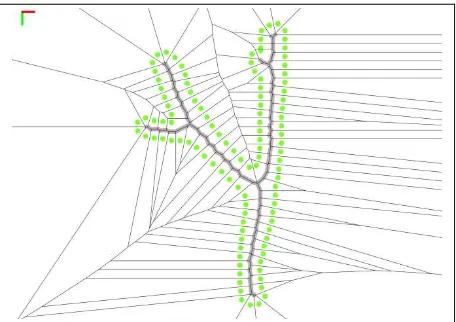
The notion that an object’s shape can be summarized by its skeleton was first formalized by (Blum, 1967) as the Medial Axis. A comprehensive overview about skeleton retrieval is given by (Biasotti et al., 2008). Here, we employ the Voronoi Diagram to obtain a skeleton graph for a given component as explained, for instance by (Ogniewicz and Ilg, 1992): The Medial Axis of a component can be closely approximated by a Voronoi Diagram that is calculated from a dense sampling of the component’s boundary, as illustrated in figure 5. An in-depth survey of Voronoi diagrams is given by (Aurenhammer and Klein, 2000). Clearly, including depth discontinuity edges in the boundary sampling, as described previously, is an essential requirement in order to obtain a skeleton reflecting the component’s actual 3D topology.
Figure 5. Voronoi Diagram from component boundary (green).
The sequence of boundary elements , which has been determined with algorithm 4, is the input for computation of the Voronoi Diagram. Subsequently, we consider only the set of Voronoi edges that is embedded within the component as depicted in figure 6a. This initial skeleton may not be one connected graph, but comprise several subgraphs due to loops in the boundary. Subgraphs are joined as follows:
1. A Delaunay triangulation is constructed using Triangle (Shewchuk, 1996) as a temporary support structure that includes all boundary segments and skeleton edges.
4. Step 2 and 3 are repeated until all subgraphs are linked and only one fully connected skeleton graph remains.
After this procedure, the initial skeleton graph consists of a single connected component. But as indicated in figure 6a, the skeleton may include a significant amount of spurious edges. As mentioned by (Biasotti et al., 2008), the Medial Axis is sensible to slight distortions of the boundary leading either to large deviations of the skeleton or to a number of additional spurious edges. Especially the boundary of trunk components is usually very noisy, which requires a filtering step.
For each Voronoi edge, the two boundary elements and , which generate this edge are known. The distance between both elements with along the boundary can be skeleton edges by a simple thresholding operation.
Residual of a skeleton edge is lower than a predefined threshold its main shape features. The result is a filtered skeleton graph as in figure 6b.
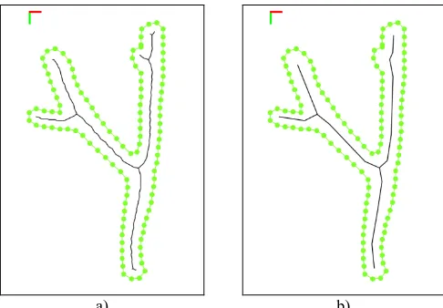
a) b)
Figure 6. Component skeleton. a) Set of embedded Voronoi edges. b) Skeleton after applying filtering and smoothing.
After retrieval of the component’s skeletal structure in 2D, the next task is the segmentation of the component itself into projection lines inevitably intersect boundary segments in order to attach them to the closest skeleton part. In its naïve formulation, the problem is reduced to a linear search over all possibilities as summarized in algorithm 7. However, the efficiency of the actual implementation can be greatly enhanced by employing a space partitioning scheme to subdivide the component boundary into several polygons. Then, a point’s location can be tested against the bounding box of each polygon. Only if the first test is successfully passed, more elaborate point-in-polygon-tests are performed to determine the exact point location in one of the candidate polygons.
Input: skeleton graph , set of points
Algorithm 7. Each point is attached to the closest skeleton part while avoiding boundary intersections with ‖ ‖ as Euclidean distance in 2D and as the projection point of onto skeleton node .
As a final step prior to calculating Principal Curves, the skeleton graph has to be split up in a set of paths. Keeping the characteristics of the polygonal line algorithm that was introduced by (Kégl, 1999) in mind, a path should be as long as possible and rather smooth regarding its curvature, while the point distribution along a path should be approximately uniform.
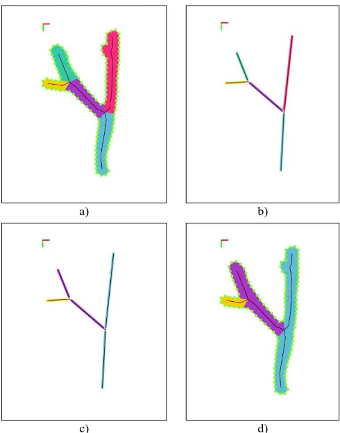
The skeleton graph consists of a set of edges and vertices . Naturally, graph leaves, i.e. vertices at skeleton ends, have a degree of 1. Most of the vertices are line vertices that have a degree of 2, and junction vertices have a degree larger than 2. Vertices of degree 2 are considered to be regular and vertices of other degrees to be irregular. We construct a new intermediary graph from the skeleton graph The intermediary graph includes all irregular vertices of , but the path formed by regular vertices and incident edges between two irregular vertices is contracted to a single edge as shown in figure 8a and 8b. Each edge in is annotated with the original path and corresponding point sets in . Similar to (Bucksch, 2011) and (Gorte, 2006), the root node is identified as the lowest skeleton vertex in the raster coordinate system. Following, the graph is traversed in depth-first fashion starting at the root. During traversal, we test edges adjacent to the current one regarding the associated path’s curvature and number of attached points. One of those adjacent child nodes that fulfills all criteria best is selected as continuation of the current path. Other child nodes that do not sufficiently fulfill all criteria are considered as separate, new paths and analogously their child nodes are tested for suitable path continuation until graph leaves are reached. Figure 8c and 8d demonstrate the result of this procedure.
2.3 Principal Curve Computation
For each extracted path, the polynomial line algorithm introduced by (Kégl, 1999) is applied to the set of attached points to obtain a Principal Curve, i.e. a compact summary of its distribution as a 3D polyline. In order to minimize the limiting effects inherent to finite floating-point arithmetic, we normalize the 3D point data prior to performing the Principal Curve computation as suggested by (Hartley and Zisserman, 2003). After this last step, the spatial structure of the component that has been our starting point is captured as the set of 3D polylines that are disjoint yet. Their adjacency relation is implicitly provided by their 2D graph counterparts in the raster.
3. EXPERIMENT SETUP AND RESULTS
a) b)
c) d)
Figure 8. Retrieval of paths. a) Component after point assignment and determination of paths between irregular vertices. b) Temporary graph; paths are contracted to edges. c) Result of path retrieval on contracted graph. d) Updated partition according to determined paths.
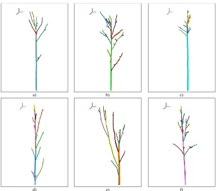
actually processed. Figure 9 demonstrates the identified components in the data raster of a single scan.
Generally speaking, the runtime of our algorithm is presently depending on the component’s size. Components that represent a small surface patch of the trunk but significant branching structure are presently processed rather quickly by our prototype implementation. Though, the point attachment to the skeleton as well as the iterative data projection and repartition structure of the polygonal line algorithm appear to be the computational bottlenecks. Computation of the skeletal structure in figure 1, which is a representative example, with 75298 points takes 40s and generates 29 polylines. Figure 10 shows further results, which complete in 4s to 113s for 13721 to 236805 points and result in 18 to 60 polylines, respectively. Processing has been performed on an Intel i5-2450m machine (8 GB RAM, MS Windows 7) with a C++ implementation. At present, the implementation is not particularly optimized. Therefore, processing of components that comprise a high number of sample points like for instance larger surface patches of trunks that were located close to the scanner takes considerably more computation time. However, especially the point assignment routine, which is currently the most time consuming step, could be replaced with a more efficient formulation in order to significantly boost performance.
The Principal Curve computation aims at finding an optimal embedding of a polyline along the centerline of an input point distribution. As a consequence, the result of the proposed strategy is a perceptually pleasing skeleton if the input component can actually be interpreted as a composite of point
densities that trace along invisible space curves. Normally, large components, which represent large fractions of branching structure and part of the trunk surface, are well reconstructed as demonstrated in figure 1 and 9, because the component can be easily recognized as tree-like structure by visual inspection. If this is not the case, for example if the component is only a small patch of trunk surface, the spatial reconstruction will not produce satisfying output because the component shape may not be reconstructable as a set of space curves at all. Unfortunately, there is no automatic mechanism to test in advance whether a shape can be summarized as a composite of space curves. Therefore, visual inspection of results is a mandatory final step.
In addition, noise in the boundary especially of trunk parts frequently leads to a number of spurious edges in the 2D skeleton estimate. Most of them are suppressed by filtering, but not all can be reliably eliminated. Consequently, remaining spurious edges degrade the retrieval of paths prior to Principal Curve computation. Similarly, the 3D topology can only be appropriately recovered as 2D skeleton if the component’s boundary is determined correctly. If depth discontinuities are not sufficiently included in the boundary description, the 2D skeleton retrieval via the Voronoi Diagram will necessarily exclude corresponding topologic features of the component shape. As a result, the overall quality of the 3D skeleton might be reduced in comparison to other component’s skeletons of the TLS data.
4. DISCUSSION
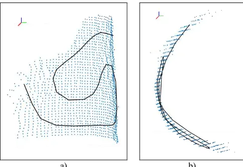
In any case, the polygonal line algorithm fits a polyline to input data. But if the data is a trunk surface patch with all eigenvalues exhibiting approximately the same magnitude, the result will be a polyline of spiral or wavy shape because this is one way to minimize the average mean square error of point distances to their parent polyline node as indicated in figure 11. Yet, eigenvalues and -vectors do not describe a component shape sufficiently. For instance, a component representing a long curvy branch may have very similar eigenvalues and -vectors as the trunk surface patch, but it can actually be well described by a 3D polyline.
Automatic, qualitative evaluation of computation results poses an open problem in skeleton retrieval. As pointed out by (Blum, 1967), the notion of a shape’s skeleton is closely related to human perception and therefore exceedingly difficult to quantify. As a consequence, we face the fact that we cannot directly assess the quality of a 3D polyline with a compact, definitive numerical description beyond an evaluation based on visual inspection.
Currently, spurious edges of the 2D skeleton estimate may interfere with retrieval of paths and therefore 3D skeleton construction. Similarly, missing topological features due to insufficient tracing of interior edges or noise effects in the range values degrade the reconstruction process. However, prior smoothing of the boundary and more fine grained analysis of the component shape by incorporating a-priori knowledge about a tree’s general structure could lead to a more reliable method for 2D skeleton construction and refinement.
Figure 9. Raster data of a single scan. Connected components are colored in gray. Components that correspond to the panels in figure 10 are highlighted in red.
a) b) c)
d) e) f)
(Raumonen et al., 2013), polylines in close proximity could be connected by testing continuity of line segments for a smooth connection and also w.r.t. ramifications. In order to obtain a full tree skeleton, a solution has to be found to connect the partial skeletons of several relevant components. In this context, the proposed strategy is not a finalized method, but rather a set of tools that needs to be investigated further to evolve into a proper method to retrieve complete tree skeletons. We conclude that the segmented data raster with 2D skeletons of its components appears to be a suitable starting point for a prospective problem solution. To sum up, we agree with (Eysn et al., 2013) that a step-wise completion of tree skeletons from results of multiple scans may result in a fitting, robust skeleton.
Explicit tree detection in scans is not required for the proposed method. In fact, trees are implicitly detected since they ought to be the only object surfaces visible from the scanner. As a result, the largest connected components are caused by trunk surfaces that are usually well represented in scans. It follows that testing whether a component contributes trunk surface could be performed during computation or as a separate post-processing step. Clearly, this constitutes a particularly attractive aspect of the proposed strategy considering large forest scenes.
a) b)
Figure 11. 3D point set represents a surface patch without a distinct principal direction; therefore, the polygonal line algorithm minimizes error by embedding a curvy polyline. a) Front view. b) Top view.
5. CONCLUSION
In this paper, we present a two stage strategy to automatically retrieve skeletal tree structures from forest scenes that have been acquired by TLS. First, we identify point clusters representing continuous surface patches in single scan range images. In addition, we trace the boundary of each connected component, which is the basis of our skeleton retrieval approach. We propose an extension of standard boundary tracing in order to trace not only a component’s silhouette but also its inner edges that are caused by depth discontinuities. Second, each component is processed separately with the objective to adequately summarize its shape as a set of 3D polygonal lines. Since the relation for each element between its 2D coordinates in the image raster and its 3D coordinates in the point cloud are known, we introduce a novel concept to obtain a skeleton by exploiting common image processing tools: A 2D skeleton from a component is generated via the Voronoi Diagram. The resulting skeleton is refined by ensuring its connectedness, filtering of spurious edges, and a smoothing
step. Subsequently, the component’s data is partitioned in such a way that each point is attached to its closest skeleton node while enforcing that the component boundary must not be disturbed by the assignment. Afterwards, the skeleton graph is split into paths. For each point cluster that is attached to a path, a Principal Curve computation is applied to describe its distribution as a 3D polygonal line. Thus, we obtain the skeletal structure of a component as a set of 3D polygonal lines.
Our proposed strategy can efficiently retrieve skeletal structures from forest scenes in leaf-less state with a comparably high tree density. Although the result is only a part of an entire tree, surface patches of trees that stand very close to the scanner may represent a significant part of the crown possibly including the entire trunk length. We believe that building a complete tree skeleton by a consistent combination of skeletal parts that are retrieved by our method from one or optionally more scans may be a more robust way to generate an adequate skeleton representation of a tree considering the high amount of occlusions that is to be expected in forest scenes.
ACKNOWLEDGMENT
Work was partly funded by DFG (Deutsche Forschungsgemeinschaft) through research grant PAK331. The Zoller+Fröhlich scanner was kindly provided by the Institute for Traffic Planning and Road Traffic (Prof. Dr. Lippold).
REFERENCES
Aurenhammer, F., and Klein, R., 1999. Voronoi Diagrams. In: Handbook of Computational Geometry, Elsevier, pp. 201–290.
Biasotti, S., Attali, D., Boissonnat, J.-D., Edelsbrunner, H., Elber, G., Mortara, M., di Baja, G.S., Spagnuolo, M., Tanase, M., and Veltkamp, R., 2008. Skeletal Structures. In: Shape Analysis and Structuring, Springer, pp. 145–183.
Blum, H., 1967. A transformation for extracting new descriptor of shape. Models for the perception of speech and visual form, 19(5), pp. 362–380.
Bucksch, A., 2011. Revealing the skeleton from imperfect point clouds. PhD Thesis, Delft University of Technology, Delft,
Côté, J.-F., Fournier, R.A., and Egli, R., 2011. An architectural model of trees to estimate forest structural attributes using terrestrial LiDAR. Environmental Modelling & Software, 26(6), pp. 761–777.
Dassot, M., Constant, T., and Fournier, M., 2011. The use of terrestrial LiDAR technology in forest science, application fields, benefits and challenges. Annals of Forest Science, 68(5), pp. 959–974.
Eysn, L., Pfeifer, N., Ressl, C., Hollaus, M., Grafl, A., and Morsdorf, F., 2013. A practical approach for extracting tree models in forest environments based on equirectangular projections of terrestrial laser scans. Remote Sensing, 5(11), pp. 5424-5448.
Gatziolis, D., Popescu, S., Sheridan, R., and Ku, N.-W., 2010. Evaluation of terrestrial LiDAR technology for the development of local tree volume equations. In: Proceedings of Silvilaser, Freiburg, Germany, pp. 197–205.
Gorte, B., 2006. Skeletonization of Laser-Scanned Trees in the 3D Raster Domain. In: Innovations in 3D Geo Information Systems. Springer, pp. 371–380.
Gorte, B., and Pfeifer, N., 2004. Structuring Laser-scanned trees using 3d mathematical morphology, In: International Archives of Photogrammetry and Remote Sensing, Vol. XXXV, Part B5, pp. 929-933.
Hartley, R.I., and Zisserman, A., 2003. Multiple View Geometry in Computer Vision. 2nd edition., Cambridge University Press, pp. 107-110 .
Hopkinson, C., Chasmer, L., Young-Pow, C., and Treitz, P., 2004. Assessing forest metrics with a ground-based scanning lidar. Canadian Journal for Forest Research, 34(3), pp. 573– 583.
Kégl, B., 1999. Principal Curves: Learning, Design, and Applications. PhD Thesis, Concordia University, Montreal, Canada.
Kégl, B., and Krzyzak, A., 2002. Piecewise linear skeletonization using principal curves. IEEE Transactions on Pattern Analysis and Machine Intelligence, 24(1), pp. 59–74.
Leica Geosystems, 2012. Cyclone pointcloud export format - Description of ASCII .ptx format. http://www.leica- geosystems.com/kb/?guid=5532D590-114C-43CD-A55F-FE79E5937CB2 (9 January.2014).
Li, H., Zhang, X., Jaeger, M., and Constant, T., 2010. Segmentation of forest terrain laser scan data. In: Proceedings of the 9th ACM SIGGRAPH Conference on Virtual-Reality Continuum and its Applications in Industry, ACM, pp. 47–54.
Livny, Y., Yan, F., Olson, M., Chen, B., Zhang, H., and El-Sana, J., 2010. Automatic Reconstruction of Tree Skeletal Structures from Point Clouds. In: ACM Transactions on Graphics (TOG), ACM, Vol. 29, no. 6, p. 151.
Maas, H.-G., Bienert, A., Scheller, S., and Keane, E., 2008. Automatic forest inventory parameter determination from terrestrial laserscanner data. International Journal of Remote Sensing, 29(5), pp. 1579–1593.
Ogniewicz, R.L., and Ilg, M., 1992. Voronoi skeletons: theory and applications. In: Proceedings of CVPR, IEEE, pp. 63–69.
Raumonen, P., Kaasalainen, M., Akerblom, M., Kaasalainen, S., Kaartinen, H., Vastaranta, M., Holopainen, M., Disney, M., and Lewis, P., 2013. Fast Automatic Precision Tree Models from Terrestrial Laser Scanner Data. Remote Sensing, 5(2), pp. 491– 520.
Schilling, A., Schmidt, A., and Maas, H.-G., 2012a. Tree Topology Representation from TLS Point Clouds Using
Depth-First Search in Voxel Space. Photogrammetric Engineering and Remote Sensing, 78(4), pp. 383–392.
Schilling, A., Schmidt, A., and Maas, H.-G., 2012b. Principal Curves for Tree Topology Retrieval from TLS Data. In: Proceedings of SilviLaser, Vancouver, Canada, pp. 16-19 .
Shapiro, L.G., and Stockmann, G.C., 2001. Binary Image Analysis. In: Computer Vision, Prentice Hall, pp. 69–75.
Shewchuk, J.R., 1996. Triangle: Engineering a 2D Quality Mesh Generator and Delaunay Triangulator. In: Applied Computational Geometry - Towards Geometric Engineering. Springer, pp.203-222.
Sonka, M., Hlavac, V., and Boyle, R., 1998. Image processing, analysis, and machine vision. 2nd edition, PWS Publishing, pp. 142–148.