COMPARISON OF 3D INTEREST POINT DETECTORS AND DESCRIPTORS
FOR POINT CLOUD FUSION
R. H¨anscha,∗, T. Webera, O. Hellwicha
a
Computer Vision & Remote Sensing, Technische University Berlin, Germany - r.haensch, [email protected]
KEY WORDS:Keypoint detection, keypoint description, keypoint matching, point cloud fusion, MS Kinect
ABSTRACT:
The extraction and description of keypoints as salient image parts has a long tradition within processing and analysis of 2D images. Nowadays, 3D data gains more and more importance. This paper discusses the benefits and limitations of keypoints for the task of fusing multiple 3D point clouds. For this goal, several combinations of 3D keypoint detectors and descriptors are tested. The experiments are based on 3D scenes with varying properties, including 3D scanner data as well as Kinect point clouds. The obtained results indicate that the specific method to extract and describe keypoints in 3D data has to be carefully chosen. In many cases the accuracy suffers from a too strong reduction of the available points to keypoints.
1. INTRODUCTION
The detection and description of keypoints is a well studied sub-ject in the field of 2D image analysis. Keypoints (also called interest points or feature points) are a subset of all points, that ex-hibit certain properties which distinguish them from the remain-ing points. Dependremain-ing on the used operator keypoints have a high information content, either radiometrically (e.g. contrast) or ge-ometrically (e.g. cornerness), they only form a small fraction of the whole data set, they can be precisely located, and their ap-pearance as well as location is robust to spatial and/or radiometric transformations.
Two dimensional keypoints have been used in many different applications from image registration and image stitching, to ob-ject recognition, to 3D reconstruction by structure from motion. Consequently, keypoint detectors are a well studied field within the 2D computer vision, with representative algorithms like SIFT (Lowe, 2004), SURF (Bay et al., 2006), MSER (Matas et al., 2004), or SUSAN (Smith and Brady, 1997)), to name only few of the available methods.
Nowadays, the processing and analysis of three-dimensional data gains more and more importance. There are many powerful algo-rithms available, that produce 3D point clouds from 2D images (e.g. VisualSFM (Wu, 2011)), or hardware devices that directly provide three-dimensional data (e.g. MS-Kinect). Keypoints in 3D provide similar advantages as they do in two dimensions. Al-though there exist considerably less 3D than 2D keypoint detec-tors, the number of publications proposing such approaches in-creased especially over the last years. Often 2D keypoint detec-tors are adapted to work with 3D data. For example, Thrift (Flint et al., 2007) extends the ideas of SIFT and SUSAN to the 3D case and also Harris 3D (Sipiran and Bustos, 2011) is an adapted 2D corner detector.
Previous publications on the evaluation of different 3D keypoint detectors focus on shape retrieval (Bronstein et al., 2010) or 3D object recognition (Salti et al., 2011). These works show that key-point detectors behave very differently in terms of execution time and repeatability of keypoint detection under noise and transfor-mations. This paper investigates the advantages and limits of 3D keypoint detectors and descriptors within the specific context of
∗Corresponding author.
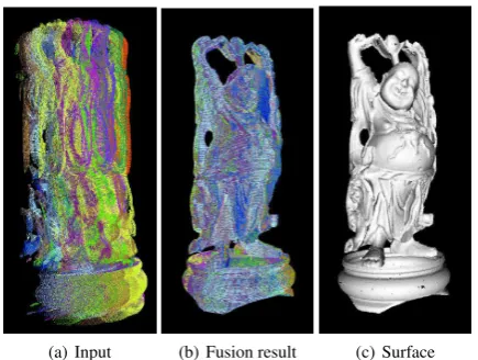
(a) Input (b) Fusion result (c) Surface
Figure 1: Point cloud fusion
point cloud fusion: Two or more point clouds are acquired from the same scene but provided within their own, local coordinate system as illustrated in Figure 1(a). The system automatically performs a chain of successive pairwise registrations and thus aligns all point clouds into a global coordinate system (see Fig-ure 1(b)). The resulting fused point cloud can then be used in subsequent tasks like surface reconstruction (see Figure 1(c)). In order to registrate two point clouds a rigid transformation con-sisting of a translation and rotation is computed by a state-of-the-art combination of a keypoint-based coarse alignment (Rusu et al., 2008) and a point-based fine alignment (Chen and Medioni, 1992, Besl and McKay, 1992, Rusinkiewicz and Levoy, 2001).
The experiments are based on ten different data sets acquired from three different 3D scenes. Different combinations of key-point detectors and descriptors are compared with respect to the gain in accuracy of the final fusion results.
2. POINT CLOUD FUSION
In a first step a fully connected graph is built. Each node corre-sponds to one of the given point clouds. Each edge is assigned with a weight, that is inverse proportional to the number of key-point-based correspondences between the two corresponding point clouds. A minimal spanning tree defines the order, in which mul-tiple pairwise fusion steps are carried out. The subsequent, suc-cessive application of the estimated transformations as well as a final global fine alignment leads to a final, single point cloud.
Figure 2: Pairwise point cloud fusion pipeline
Figure 2 shows the processing chain to align two point clouds as it is used in this paper. Both acquired point clouds are prepared by several filters that reject large planes, isolated points, as well as points far away. The prepared point clouds are used to com-pute a rigid transformation matrix that consists of a rotation and a translation. The transformation matrix is applied to the original source point cloud to align it with the original target point cloud into a common coordinate system.
The alignment is based on a first coarse feature-based alignment and a subsequent fine point-based alignment using ICP. The fea-ture-based alignment uses the computed feature descriptors of the points in both point clouds to establish point correspondences tween similar points. From these set of point correspondences be-tween both point clouds, a transformation is computed that aligns the corresponding points in a least-squares sense. This coarse pre-alignment is necessary, since ICP in the second step performs only a local optimization and can only correctly registrate two point clouds with small differences in rotation and translation.
3. 3D KEYPOINT DETECTION
An explicit keypoint estimation reduces the set of points for which point descriptors have to be calculated and decreases the number of possible correspondences. In this paper Normal Aligned Ra-dial Feature (NARF) and a 3D adaption of SIFT are used as they represent two interesting as well as complementary approaches to detect 3D keypoints in point clouds.
3.1 NARF
The Normal Aligned Radial Feature (NARF) keypoint detector (Steder et al., 2011) has two major characteristics: Firstly, NARF extracts keypoints in areas where the direct underlying surface is stable and the neighborhood contains major surface changes. This causes NARF keypoints to be located in the local environ-ment of significant geometric structures and not directly on them. According to the authors this characteristic leads to a more ro-bust point descriptor computation. Secondly, NARF takes ob-ject borders into account, which arise from view dependent non-continuous transitions from the foreground to the background. Thus, the silhouette of an object has a profound influence on the resulting keypoints.
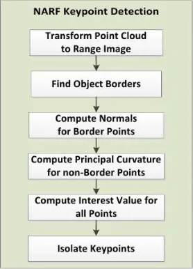
Figure 3: NARF keypoint computation
Figure 3 shows the major steps of the NARF keypoint detection. The point cloud is transformed into a range image to perform a heuristic-based detection of object borders. The range values within a local neighborhood of sizesaround every image pointp are ordered by their 3D distances to p. From this ordered set dM is selected as mean distance withdM = (0.5·(s+ 1))2.
Four score valuessright,sbottom,slef t, andstopare computed
by Equation 1, which represent the possibility of a border in the corresponding direction. The pointpis marked as a border point, if the score of any direction exceeds a specified threshold.
si= max
0,1−dM
di
(1)
wherediis the average distance frompto its next three direct
point neighbors in directioni ∈ {right, bottom, lef t, top}of the range image. The normal vector of border points and the principal curvature of non-border points are used to detect in-terest points. They are determined by the main directionαof surface change and a weightw. The normal vector of a border pointpis projected onto a plane perpendicular to the vector be-tween the viewpoint andp, where it is used to compute the main directionα. The weight is set tow = 1. In the case of a non-border pointp, the direction of maximal curvature is projected onto a plane perpendicular to the vector between the viewpoint andp. The resulting angle defines the main directionαand the corresponding curvature is set as the weightw.
An interest scoreI(p)is defined for every pointp, which is based on all neighboring points{n0, ..., nk}ofpwithin a radius ofσ,
which do not have a border in between:
I(p) =I1(p)·I2(p) (2)
I1(p) = min
i
1−wnimax
1−10· kp−nik
σ ,0
(3)
I2(p) = max
i,j f(ni)·f(nj) 1− |cos αni−αnj
| (4)
f(n) = s
wn
1−
2· kp−nk
σ −0.5
(5)
Figure 4: Point cloud with NARF keypoints
3.2 3D-SIFT
The Scale Invariant Feature Transform (SIFT, (Lowe, 2004)) orig-inally developed for 2D images was adapted by the community of the Point Cloud Library (PCL) to 3D point clouds (Rusu and Cousins, 2011) by replacing the role of the intensity of an pixel in the original algorithm by the principal curvature of a point within the 3D cloud.
Figure 5: 3D-SIFT keypoint computation
Figure 5 gives an overview of the major steps of the 3D-SIFT keypoint detection. The 3D-SIFT keypoints are positioned at the scale-space extrema of the Difference-of-Gaussian (DoG) func-tion. The used Gaussian scale-space is created by downsampling with voxelgrid filters of different sizes and a blur filter by per-forming a radius search for each pointpand then computing the new intensity as weighted average of the found neighbors. For each two adjacent point clouds a new DoG point cloud is com-puted. All points of the resulting DoG point cloud have the same position as in the involved point clouds, but their intensity val-ues represent the difference of the intensity valval-ues of the original points. The DoG is a good approximation of the scale-normalized Laplacian of the Gaussian function, which can be used to gener-ate stable keypoints. A point is marked as keypoint candidgener-ate if it has the highest or lowest DoG value among all itsknearest point neighbors within its own, as well as in its lower and upper DoG point cloud neighbors. Finally, all keypoints in areas with low curvature values are rejected to get stable results. Figure 6 shows the resulting keypoints of 3D-SIFT when applied to an example point cloud.
4. 3D KEYPOINT DESCRIPTION
3D keypoint descriptors deliver a description of the local environ-ment of a point within the point cloud. This description often only depends on geometric characteristics. But there are also point de-scriptors, which additionally use color information. Points in dif-ferent point clouds with a similar feature descriptor are likely to
Figure 6: Point cloud with 3D-SIFT keypoints
represent the same surface point. By establishing those point cor-respondences, a transformation is estimated that aligns the two point clouds. A point descriptor must deliver an accurate and ro-bust description of the local environment of the point to avoid wrong matches which decrease the accuracy of the alignment. A good feature descriptor should be robust against noise, fast to compute, fast to compare, and invariant against rotation and translation of the point cloud (Lowe, 2004).
In (Arbeiter et al., 2012) the object recognition capabilities of different feature descriptors are evaluated. The work of (Salti et al., 2011) shows that not all feature descriptor and keypoint detector combinations deliver good results. In this paper Point Feature Histograms (PFH) and Signature of Histograms of Ori-entations (SHOT) with their variants are used. They are chosen because they represent common feature descriptors and behave differently in computation time and accuracy.
4.1 Point Feature Histograms
Figure 7: PFH descriptor computation for one point
The Point Feature Histograms (PFH) descriptor was developed in 2008 (Rusu et al., 2008). Besides the usage for point matching, the PFH descriptor is used to classify points in a point cloud, such as points on an edge, corner, plane, or similar primitives. Figure 7 shows an overview of the PFH computation steps for each pointp in the point cloud.
Figure 8: Darboux frame between a point pair [Rus09]
angle between its normal and the connecting line between the point pairpsandpt. Ifns/tis the corresponding point normal,
the Darboux frameu,v,wis constructed as follows:
u = ns (6)
v = u× pt−ps kpt−psk
(7)
w = u×v (8)
Three angular valuesβ,φ, andθare computed based on the Dar-boux frame:
β = v·nt (9)
φ = u·(pt−ps)/d (10)
θ = arctan(w·nt, u·nt) (11)
d = ||pt−ps|| (12)
wheredis the distance betweenpsandpt.
The three angular and the one distance value describe the relation-ship between the two points and the two normal vectors. These four values are added to the histogram of the pointp, which shows the percentage of point pairs in the neighborhood ofp, which have a similar relationship. Since the PFH descriptor uses all possible point pairs of thekneighbors ofp, it has a complexity ofO(n·k2)
for a point cloud withnpoints.
The FPFH variant is used to reduce the computation time at the cost of accuracy (Rusu, 2009). It discards the distance dand decorrelates the remaining histogram dimensions. Thus, FPFH uses a histogram with only3·bbins instead ofb4
, wherebis the number of bins per dimension. The time complexity is reduced by the computation of a preliminary descriptor value for each pointp by using only the point pairs betweenpand its neighbors. In a second step it adds the weighted preliminary values of the neigh-bors to the preliminary value of each point. The weight is defined by the Euclidean distance frompto the neighboring point. This leads to a reduced complexity ofO(nk)for the FPFH descriptor.
The PCL community also developed the PFHRGB variant (PCL, 2013), which additionally uses the RGB values of the neighbor-ing points to define the feature descriptor. The number of bins of the histograms is doubled. The first half is filled based on the point normals. The second half is computed similar to the description above, but uses RGB values of the points instead of their 3D information.
4.2 Signature of Histograms of Orientations
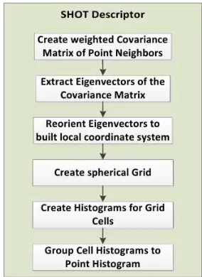
In 2010 an evaluation of existing feature descriptors led to the conclusion, that one of the hardest problems of the evaluated de-scriptors is the definition of a single, unambiguous and stable lo-cal coordinate system at each point (Tombari et al., 2010). Based on this evaluation the authors proposed a new local coordinate system and the Signature of Histograms of Orientations (SHOT) as a new feature descriptor (Tombari et al., 2010). An overview of the computation steps for each pointpin the point cloud is visualized in Figure 9. The first three steps consist of the compu-tation of a local coordinate system atp. Thenneighborspiof a
pointpare used to compute a weighted covariance matrixC:
C= 1
n
n
X
i=1
(r− kpi−pk)·(pi−p)·(pi−p)T (13)
whereris the radius of the neighborhood volume.
Figure 9: SHOT descriptor computation for one point
An eigenvalue decomposition of the covariance matrix results in three orthogonal eigenvectors that define the local coordinate sys-tem atp. The eigenvectors are sorted in decreasing order by their corresponding eigenvalue asv1,v2, andv3, representing theX-,
Y-, andZ-axis. The direction of theX-axis is determined by the orientation of the vectors frompto the neighboring pointspi:
X =
v1 , if |S+x| ≥ |Sx−|
−v1 , otherwise. (14)
S+
x = {pi|(pi−p)·v1≥0} (15)
S−
x = {pi|(pi−p)·v1<0} (16)
The direction of theZ-axis is similarly defined. The direction for theY-axis is determined via the cross product betweenX and Z. This local coordinate system is used to divide the spatial en-vironment ofpwith an isotropic spherical grid. For each pointpi
in a cell the angleξi = pi·pis computed between the points
normal and the normal ofp. The local distribution of angles is subsequently described by one local histogram for each cell.
If the spherical grid containskdifferent cells with local histograms and each histogram containsbbins, the resulting final histogram containsk·bvalues. These values are normalized to sum to one in order to handle different point densities in different point clouds.
Color-SHOT (Tombari et al., 2011) includes also color informa-tion. Each cell in the spherical grid contains two local histograms. One for the angle between the normals and one new histogram, which consists of the sum of absolute differences of the RGB values between the points.
5. PERSISTENT FEATURES
Persistent features are another approach to reduce the number of points in a cloud. It is published together with the PFH descriptor and is strongly connected to its computation (Rusu et al., 2008).
In a first step the PFH descriptors are computed at multiple in-creasing radiiri for all points of the point cloud. A mean
his-togramµiis computed from all PFH point histograms at radiusri.
For each point histogram of radiusrithe distance to the
corre-sponding mean histogramµiis computed. In (Rusu et al., 2008)
used, since it led to better experimental results within the here discussed application scenario. Every point whose distance value in one radius is outside the interval ofµi±γ·σiis marked as a
persistent point candidate. Theγvalue is a user specified value andσiis the standard deviation of the histogram distances for
ra-diusri. The final persistent point set contains all points, which
are marked at two radiiriandri+1as persistent point candidates.
Figure 10 shows an example of the resulting point cloud after a persistent feature computation. No additional filtering steps are used in this example and all111,896points of the original point cloud are used. The FPFH descriptor was computed at three dif-ferent radii of3.25cm,3.5cm, and3.75cmandγ= 0.8.
Figure 10: Point cloud before (left) and after (right) the persistent features computation
6. EXPERIMENTS
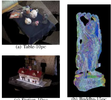
This section compares the quantitative as well as qualitative per-formance of different keypoint detector and descriptor combi-nations. Three different scenes are used to create ten 3D test datasets, which are used in the following experiments. While the Happy Buddha model was generated by a laser scan, the table and station test sets were acquired by the Microsoft Kinect device. If a test set name has the suffixn-ks, the individualnpoint clouds are acquired by different kinect sensors, while the suffixn-pc in-dicates that the same sensor at different positions was used.
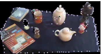
Table scenes as in Figure 11(a) are common test cases for point cloud registration methods. Each of the individual point clouds used here contains approximately307,200points.
The station scene (see Figure 11(c)) contains a model of a train station. The major problem regarding the fusion algorithm is its symmetric design. Two test sets were created from this scene. Each point cloud contains approximately307,200points.
The third scene is the Happy Buddha model shown in Figure 11(b) of the Stanford 3D Scanning Repository (Stanford, 2013). These point clouds were created with a laser scanner and a rotating ta-ble. Compared to the point clouds of a Kinect sensor, the laser scans contain little noise and are more accurate. But the resulting point clouds contain no color information. Four point cloud test sets were created from the Happy Buddha dataset. The test sets Buddha-0-24, Buddha-0-48, and Buddha-0-72contain two point clouds. These three test sets contain the point cloud scan at the 0◦position of the rotating table and the point cloud at the24◦, 48◦, and72◦ position, respectively. The test set Buddha-15pc contains15point clouds from a360◦rotation. Each point cloud of the Happy Buddha laser scan contains about240,000points.
6.1 Quantitative Comparison of Keypoint Detectors
Both keypoint detectors presented in Section 3. use different ap-proaches to define interesting points in a point cloud. The NARF detector converts the captured point cloud into a 2D range image and tries to find stable points, which have borders or major sur-face changes within the environment. This results in keypoints,
(a) Table-10pc
(b) Buddha-15pc
(c) Station-10pc
Figure 11: Example datasets
which depend on the silhouette of an object. In contrast, 3D-SIFT uses scale space extrema to find points, which are likely to be recognized even after viewpoint changes. The user specified parameters of both methods are empirically set to values, which led to reasonable results in all test cases. The 3D-SIFT detector has more parameters and is slightly more complex to configure.
The resulting set of keypoints differ significantly. Examples of NARF and 3D-SIFT keypoints are shown in Figure 4 and Fig-ure 6, respectively. In both cases the same input point cloud with111,896points is used. Table 1 summarizes, that the 3D-SIFT detector marks more keypoints than the NARF detector. Both keypoint detectors mostly ignore the center of the table plane and mark many points at the table border. In addition, 3D-SIFT strongly responds to object borders and major surface changes, while NARF mostly reacts to keypoints near object bor-ders. The 3D-SIFT detector has a considerably higher runtime than the NARF detector. The median runtime of NARF for this point cloud is about0.05sec, while 3D-SIFT needs about2sec.
NARF 3D-SIFT
number of keypoints 146 2838 median runtime 0.046sec 1.891sec
Table 1: Quantitative comparison of NARF and 3D-SIFT results
6.2 Quantitative Comparison of Keypoint Descriptors
The PFH and SHOT descriptor mainly differ in their way to de-fine local coordinate systems. Both feature descriptors have in common, that they use the differences of point normals in the neighborhood to create a feature histogram as descriptor. The free parameters are set to the proposed values of the original pub-lications of the algorithms.
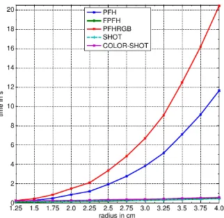
Figure 12: Runtime of point descriptors
many bins, it is more expensive to find the most similar point in another point cloud. For a fast matching procedure, less bins are preferable. The FPFH descriptor is best suited for time-crucial applications, since it is not only fast to compute, but also consists only of33histogram bins per point.
6.3 Comparison of the Detector-Descriptor-Combinations
All possible keypoint detector and descriptor combinations are used to fuse the point clouds of all described test sets by the above explained fusion pipeline. All tests are performed with and without the persistent feature computation as well as with10 and100iterations of the ICP algorithm. The persistent features are computed using the FPFH descriptor at three different radii of3.25cm, 3.5cm, and3.75cmand an γ = 0.8. The varia-tion of the number of ICP iteravaria-tions allows to observe the impact of ICP and to deduce the quality of the feature-based alignment. All remaining parameters of the point cloud fusion algorithm are set to reasonable values for each test scene. Due to the reason that the Happy Buddha scene contains only a single object with little noise, the distance, plane, and outlier filter are skipped for the corresponding test sets. As the PFHRGB and Color-SHOT descriptor use color information, which are not available for the Happy Buddha scene, the total number of tests in the correspond-ing cases is six. In all other cases, all ten tests are performed.
For the first part of the following discussion, a rather subjec-tive performance measure is used: A result of a test is classified as correct, if it contains no visible alignment error. The follow-ing tables contain the aggregated results of the performed tests. Tables 2-3 show the percentage of correct results with10and 100ICP iterations, respectively, as well as the overall time of the fusion process. The top part of each table contains the re-sults without and the lower part with the computation of persis-tent features. Each row contains the results of a different feature descriptor and each column represents the results with the speci-fied feature detector. Column “None” represents the case, when no keypoint detector is applied.
The most important conclusion of these results is, that the pro-posed fusion pipeline using the FPFH descriptor with no feature detection and without the computation of persistent features out-performs all other tested combinations. This combination is able to produce correct results for all test sets with100iterations of ICP and has a comparatively low computation time. At almost all cases, the combinations using no feature detector have a bet-ter or at least equal success rate than combinations using NARF or 3D-SIFT. There are different reasons possible why feature de-tectors lead to inferior results. One important aspect is that the
Without persistent features None NARF 3D-Sift FPFH 90.0% 00.0% 30.0%
0.82s 0.50s 0.74s PFH 70.0% 10.0% 40.0% 2.08s 0.50s 0.87s
PFHRGB 66.7% 00.0% 33.3%
5.27s 0.55s 1.57s SHOT 20.0% 00.0% 10.0% 22.94s 0.53s 1.82s Color-SHOT 00.0% 00.0% 16.7% 105.69s 0.70s 8.87s With persistent features None NARF 3D-Sift FPFH 40.0% 10.0% 10.0%
1.17s 1.00s 1.05s PFH 60.0% 10.0% 40.0% 1.70s 0.99s 1.17s
PFHRGB 16.7% 33.3% 16.7%
2.99s 0.69s 1.21s SHOT 20.0% 20.0% 00.0% 11.26s 1.06s 1.62s Color-SHOT 16.7% 00.0% 16.7% 50.72s 0.83s 3.91s
Table 2: Runtime and subjective results (10 ICP iterations)
Without persistent features None NARF 3D-Sift FPFH 100.0% 20.0% 40.0%
1.56s 1.69s 1.75s
PFH 90.0% 30.0% 50.0% 2.87s 1.79s 1.84s
PFHRGB 66.7% 33.3% 33.3%
6.53s 2.31s 2.92s SHOT 50.0% 10.0% 20.0% 24.13s 1.82s 3.15s Color-SHOT 50.0% 16.7% 33.3% 130.33s 2.21s 10.44s
With persistent features None NARF 3D-Sift FPFH 50.0% 30.0% 20.0%
1.71s 1.60s 1.85s PFH 60.0% 30.0% 50.0% 2.18s 1.66s 1.68s
PFHRGB 33.3% 33.3% 16.7%
3.85s 1.43s 2.07s SHOT 20.0% 20.0% 20.0% 11.79s 1.78s 2.25s Color-SHOT 66.7% 00.0% 33.3% 56.64s 1.97s 5.04s
Table 3: Runtime and subjective results (100 ICP iterations)
global point cloud graph used in the fusion process produces bet-ter point cloud pairs for the pairwise registration, if more points are used. Especially the 3D-SIFT feature detector performs well at test sets with only two point clouds, but failed at nearly all test sets with more than two point clouds. The NARF detector shows a similar effect.
blurred object boundaries due to its working principle and a ro-tation of a single object can result into major silhouette changes. This leads to very different keypoint positions between the point clouds and to a bad initial alignment of the point clouds. Increas-ing the number of ICP iterations sometimes leads to the correct result. Using the optional persistent feature step leads in nearly all combinations with the NARF detector to better or at least equal success rates. The reason is that the persistent feature computa-tion generates more homogenous object borders, which lead to less different NARF keypoint positions between the point clouds.
Using a descriptor of the PFH family delivers for most combi-nations a higher success rate than combicombi-nations using SHOT or Color-SHOT. Based on the results of the Happy Buddha scene it can be concluded that at least the FPFH descriptor and PFH descriptor tolerate larger viewpoint changes than the SHOT de-scriptor. In contrast to the PFH and FPFH descriptor, the SHOT descriptor is not able to produce a correct result at the Buddha-0-72test set for any combination. From the used test sets, the Buddha-15pcis the most challenging. The algorithm needs to create14point cloud pairs from the360◦scan in order to fuse all point clouds. If one point cloud pair does not have a suf-ficiently large overlap, the fusion result will be incorrect. The FPFH and PFH descriptor in combination with no persistent fea-tures computation and without a keypoint detection are able to find all14directly adjacent point cloud pairs and produce a cor-rect fusion result. The SHOT descriptor leads to one not dicor-rectly adjacent pair of point clouds, but still produced the correct result with100ICP iterations. All other combinations do not lead to adequate point cloud pairs and produced wrong fusion results.
The results of the Table-2ksand Table-4kstest sets reveal one problem of the PFHRGB and the Color-SHOT feature descrip-tors. These sets contain significant color differences between the point clouds, which were acquired by different Kinect devices. Except for one combination, the PFHRGB and the Color-SHOT feature descriptors produced incorrect results. The feature de-scriptor variants, which only use the geometry but no color in-formation, delivered correct results for more combinations. As a consequence, the RGB cameras of different Kinect devices should be calibrated, if the feature descriptor uses color information.
Tables 2-3 also contain the mean runtimes in seconds of all tests with10and100ICP iterations, respectively. As test platform a Windows 864bitsystem with a XeonE3-1230V2processor was used. The values in these tables are intended to show the relative runtime changes between the different test parameters. Not ap-parent in these tables is the increase in computation time due to a larger number of point clouds or more points per point cloud.
The persistent feature computation is able to notably decrease the computation speed, especially if there are many points and a feature descriptor with many dimensions is used. This is the case at pipeline combinations, which are using no keypoint detec-tor or the 3D-SIFT feature detecdetec-tor together with the PFHRGB, SHOT, or Color-SHOT descriptor. Under these circumstances the point descriptor computation and the point descriptor match-ing between the point clouds need more computation time than the persistent feature computation. But except for several of the NARF detector combinations and for the combination of the Color-SHOT descriptor without a feature detector, the computation of persistent features mostly decreases the success rate. The choice of an additional persistent feature computation step is a trade-off between a faster computation speed and a higher success rate. A similar trade-off is made by the selection of the number of ICP iterations. There is no test case, where100ICP iterations led to
a wrong result, if the result was already correct at10ICP iter-ations. But there are many cases with an increased success rate with more ICP iterations. Especially the combinations using the NARF keypoint detector and without the persistent feature com-putation benefit from more ICP iterations. The average runtimes in nearly all cases show, that more dimensions of the used point descriptor lead to a higher computation time. One reason is, that a high dimensional k-d tree probably degenerates and loses its speed advantage. For example, Color-SHOT uses1280 dimen-sions to describe a point and most of the computation time is spent at the correspondence point computation. Therefore, a key-point detector or the persistent feature computation can reduce the computation time for point descriptors with many dimensions.
Scene max. MSE max. MCE
Table-2ks <0.01% 0.08% Buddha-0-24 <0.01% <0.01% Buddha-0-48 <0.01% 0.02% Buddha-0-72 <0.01% 0.02% Buddha-15pc <0.01% 0.01%
Table 4: Maximum error of correct results
In order to obtain a more objective impression about the accu-racy of the obtained results, all cases defined above as ”correct” are compared to reference results. This comparison allows qual-itative statements about the fusion accuracy. Table 4 shows the largest mean squared error (MSE) and the largest maximum cor-respondence error (MCE) of the correct results of each test set. They represent the mean and the maximum nearest point neigh-bor distance between all points of the fusion result and the refer-ence result and are expressed as percentage of the maximum point distance of the reference result. This enables an easier compar-ison of the individual results. At the Buddha scene, the public available reference transformations from the Stanford 3D Scan-ning Repository are used to create the reference result. The refer-ence results of the Station and Table scene are created by manual selection of corresponding points and additional ICP and global registration steps using MeshLab. Compared to the error values of the other test sets, the correct Table scene test results contain a large error with a MSE up to0.06%and a MCE up to3.54%. This is caused by the large amount of noise within this test scene, which allows a wider difference for correct results. The high-est error of the remaining thigh-est results has a MSE value less than 0.01%and a MCE of0.05%.
7. CONCLUSION
This paper discussed the benefits and limits of different keypoint detector and descriptor combinations for the task of point cloud fusion. An automatic multi point cloud fusion processing chain computes a transformation for each point cloud, which is based on a coarse feature-based alignment and a subsequent fine align-ment by ICP.
computed for the selected subset of the point cloud. This paper uses point descriptors from the PFH and SHOT families.
Evaluation results show that the proposed pipeline is able to pro-duce correct fusion results at complex scenes and360◦ object scans. The best performing pipeline configuration with respect to the tradeoff between accuracy and speed uses the FPFH descrip-tor and no additional persistent feature or keypoint computation. Both pipeline steps mainly lead to worse fusion results, but re-duce the computation time if a complex feature descriptor is used.
A reason for the decreased accuracy is that the heuristic of the global point cloud graph generates better point cloud pairs, if more points are available. If a point cloud contains less 3D in-formation (ie. points), it is harder to match it with another point cloud based on similarities between the respective 3D structures.
The NARF keypoint detector converts the point cloud into a range image and uses object borders to find keypoints. NARF key-points are fast to compute, but the resulting keypoint subset is too small in order to use them in the global point cloud graph. Ad-ditionally, the detected NARF keypoints are unstable because the Kinect sensor produces blurred object borders due to its working principle. As result, the NARF keypoint detector is only usable to align one point cloud pair with enough ICP iterations. Using more than two point clouds as input for the point cloud fusion process with the NARF keypoint detector leads only in rare cases to a correct result. In comparison to the NARF keypoint detector, the 3D-SIFT keypoint detector needs more computation time, but also leads to better fusion results. It results in a larger set of key-point than NARF, which helps the heuristic of the global key-point cloud graph to find the best point cloud pairs. Nevertheless, the point cloud fusion process is more often successful, if the key-point detection is skipped during the key-point cloud preparation.
Point descriptors of the PFH family are faster to compute and more robust against viewpoint differences than descriptors of the SHOT family. The PFH family also delivers more reliable infor-mation about the most overlapping point cloud pairs during the global point cloud graph computation. As a consequence, the SHOT descriptors lead to inferior fusion results. The PFHRGB and Color-SHOT point descriptor are variants, which use the ge-ometry as well as the point colors to describe a point. If the input point clouds are captured by different Kinect sensors and a color-based descriptor is used, the RGB cameras should be calibrated beforehand. Otherwise, too different point cloud colors lead to wrong fusion results.
REFERENCES
Arbeiter, G., Fuchs, S., Bormann, R., Fischer, J. and Verl, A., 2012. Evaluation of 3D feature descriptors for classification of surface geometries in point clouds. In: Intelligent Robots and Systems (IROS), 2012 IEEE/RSJ International Conference on, pp. 1644–1650.
Bay, H., Tuytelaars, T. and Gool, L. V., 2006. Surf: Speeded up robust features. In: In ECCV, pp. 404–417.
Besl, P. J. and McKay, N. D., 1992. Method for registration of 3-D shapes. In: Robotics-DL tentative, International Society for Optics and Photonics, pp. 586–606.
Bronstein, A. M., Bronstein, M. M., Bustos, B., Castellani, U., Crisani, M., Falcidieno, B., Guibas, L. J., Kokkinos, I., Murino, V., Ovsjanikov, M., Patan´e, G., Sipiran, I., Spagnuolo, M. and Sun, J., 2010. SHREC’10 track: feature detection and descrip-tion. In: Proceedings of the 3rd Eurographics conference on 3D
Object Retrieval, EG 3DOR’10, Eurographics Association, Aire-la-Ville, Switzerland, Switzerland, pp. 79–86.
Chen, Y. and Medioni, G., 1992. Object modelling by registration of multiple range images. Image and Vision Computing 10(3), pp. 145–155.
Flint, A., Dick, A. and Hengel, A. v. d., 2007. Thrift: Local 3D Structure Recognition. In: Digital Image Computing Techniques and Applications, 9th Biennial Conference of the Australian Pat-tern Recognition Society on, pp. 182–188.
Lowe, D. G., 2004. Distinctive image features from scale-invariant keypoints. International journal of computer vision 60(2), pp. 91–110.
Matas, J., Chum, O., Urban, M. and Pajdla, T., 2004. Robust wide-baseline stereo from maximally stable extremal regions. Image and Vision Computing 22(10), pp. 761 – 767. British Ma-chine Vision Computing 2002.
PCL, 2013. Point Cloud Library. http://www.pointclouds.org. last visit: 21.11.2013.
Rusinkiewicz, S. and Levoy, M., 2001. Efficient variants of the ICP algorithm. In: Proceedings of Third International Confer-ence on 3D Digital Imaging and Modeling, 2001., IEEE, pp. 145– 152.
Rusu, R. B., 2009. Semantic 3D Object Maps for Everyday Ma-nipulation in Human Living Environments. PhD thesis, Technis-che Universitt M¨unTechnis-chen.
Rusu, R. B. and Cousins, S., 2011. 3D is here: Point Cloud Library (PCL). In: IEEE International Conference on Robotics and Automation (ICRA), Shanghai, China.
Rusu, R., Blodow, N., Marton, Z. and Beetz, M., 2008. Align-ing point cloud views usAlign-ing persistent feature histograms. In: Intelligent Robots and Systems, 2008. IROS 2008. IEEE/RSJ In-ternational Conference on, pp. 3384–3391.
Salti, S., Tombari, F. and Di Stefano, L., 2011. A Performance Evaluation of 3D Keypoint Detectors. In: 3D Imaging, Modeling, Processing, Visualization and Transmission (3DIMPVT), 2011 International Conference on, pp. 236–243.
Sipiran, I. and Bustos, B., 2011. Harris 3D: a robust extension of the Harris operator for interest point detection on 3D meshes. The Visual Computer 27(11), pp. 963–976.
Smith, S. M. and Brady, J. M., 1997. SUSAN - A new approach to low level image processing. International journal of computer vision 23(1), pp. 45–78.
Stanford, 2013. Stanford 3D Scanning Repository. http://graphics.stanford.edu/data/3Dscanrep. last visit: 21.11.2013.
Steder, B., Rusu, R., Konolige, K. and Burgard, W., 2011. Point feature extraction on 3D range scans taking into account object boundaries. In: Robotics and Automation (ICRA), 2011 IEEE International Conference on, pp. 2601–2608.
Tombari, F., Salti, S. and Di Stefano, L., 2011. A combined texture-shape descriptor for enhanced 3D feature matching. In: Image Processing (ICIP), 2011 18th IEEE International Confer-ence on, pp. 809–812.
Tombari, F., Salti, S. and Stefano, L., 2010. Unique Signatures of Histograms for Local Surface Description. In: K. Daniilidis, P. Maragos and N. Paragios (eds), Computer Vision ECCV 2010, Lecture Notes in Computer Science, Vol. 6313, Springer Berlin Heidelberg, pp. 356–369.