Agustriyanto Control structure selection for 2006

(1)

CONTROL STRUCTURE SELECTION FOR THE ALSTOM GASIFIER BENCHMARK PROCESS USING GRDG ANALYSIS

Rudy Agustriyanto1,2, Jie Zhang1

1_{School of Chemical Engineering and Advanced Materials, University of Newcastle,}

Newcastle upon Tyne NE1 7RU, UK

2

University of Surabaya, Indonesia

Abstract: The objective of this work is to explore the disturbance rejection capability of possible multi-loop control structures for the ALSTOM gasifier benchmark process and selecting the appropriate control structure. Generalized Relative Disturbance Gain (GRDG) analysis is used for control structure determination. In order to carry out GRDG analysis, process models in the form of transfer functions are obtained from the discrete time models identified using the Output-Error (OE) method for system identification. Models identified with the OE method can provide accurate long range prediction (or simulation) performance and, hence, lead to accurate transfer function models. The GRDG analysis results clearly show that the baseline controller proposed by Asmar et al. (Asmar et al., 2000) is the favoured multi-loop control structure among their initial designs. This study provides explanation for the reason behind the impressive performance of the ALSTOM baseline controller that is not available before.

Keywords: ALSTOM Gasifier, Relative Disturbance Gain Array, Plantwide Control, Process Control.

1. INTRODUCTION

In 1997 the ALSTOM Power Technology Centre issued an open challenge to the UK academic control community, which addressed the control of a Gasifier plant (Dixon et al., 2000). The ‘challenge information pack’ included three linear models (obtained from ALSTOM’s comprehensive non-linear model of the system). Full detail of this challenge can be found in reference (Burnham et al., 2000; Dixon et al., 2000).

Among the approaches that have been proposed to solve this challenging problem, Asmar et al. (Asmar et al., 2000) provide a relatively simple controller structure but with excellent control performance. It only fails in its regulation task during one of the six pressure disturbance tests. Later this structure was adopted and used as a baseline controller in the second round of ALSTOM benchmark challenge (Dixon and Pike, 2004), where the nonlinear simulation programme for the process is provided. Unfortunately, up to now there have been no formal

analysis on why the baseline control structure gives good performance and no theoretical analysis in a systematic manner have been given to explain the evolution from the initial design towards the final solution (baseline controller).

Some other more complex control approaches proposed for this benchmark process include multi-objective optimization (Griffin et al., 2000) and multivariable proportional-integral (PI) controller tuning methodology based on multi-objective optimization (Liu et al., 2000). Taylor et al. (Taylor et al., 2000) proposed multivariable proportional-integral plus (PIP) controllers. Rice et al. (2000) used model predictive control to control this process. A sequential loop selection technique combined with high frequency decoupling is applied to the benchmark process (Munro et al., 2000).

(2)

simulation programme. Section 4 provides GRDG analysis for control structure determination. The paper ends with some conclusions.

2. GENERALIZED RELATIVE

DISTURBANCE GAIN (GRDG)

Based on the process and disturbance transfer functions, Stanley et al. (Stanley et al., 1985) proposed the relative disturbance gain (RDG) for analysing the disturbance rejection capability in multi-loop control. The RDG overcomes one of the limitations of the RGA (relative gain array) by allowing disturbances to be included in an operability analysis.

For the following multivariable process:

d

G

u

G

y

=

.

+

d

.

(1)

where y is the output, u is the manipulated variable and d is the disturbance. The ith element of RDG is defined as (Stanley et al., 1985) :

≠













∂













∂

=

uij yi i

y i

i

d

u

d

u

j

,

β

(2)

The term in the numerator denotes the change in the

manipulated variable ui needed for perfect

disturbance rejection. The term in the denominator

represents the change in manipulated variable ui

when one of the output yi is kept perfect. Equation

(2) can be rearranged and the vector of RDG can be expressed as:

{

G

,

G

_diag

,

Gd

}

(

G

1

G

_d

)

.

RDG

=

− ∅

(

( )

G

_diag −1

G

_d

)

.

(3)

where ∅denotes element by element division.

The concept of RDGA is very similar to RGA (Bristol, 1966) except that RDGA emphases on load disturbance rejection. Since RDG is pairing

dependent (β

i depends on the input-output pairing),

an n×n array can be constructed after going through

n possible pairings (forming n vectors). Therefore, an

augmented version of relative disturbance gain

β

ij

can be defined and a matrix can be formed. The matrix RDGA (B) is defined as (Chang and Yu, 1992):

u

₁

u

₂

...

u

_n

B =

n nn n

n

y

n

.

...

.

...

.

...

2 1

1

2 22

21 12

11 1













β

(4)

The ijth entry,

β

ij, corresponds to the RDG when the

ith output is paired with the jth input. Notice that,

since the vector Gd is involved in the computation of

β

ij, corresponding changes in Gd have to be made in

permutation in the outputs in the matrix G.

In a matrix notation, the B matrix can be promptly calculated from:

[

G

diag

Gd

]

[

diag

(

G

d

)

]

B

=

−1

.

(

)

−1

.

−1 ₍₅₎

where diag(.) transforms a vector (.) into a matrix with elements put on the corresponding diagonal positions, that is, the ith element of a vector (.) is put in the iith entry of a matrix. Equation (5) simplifies the computation of RDGA.

An interaction measure GRDG is defined to evaluate the load effect under a specific controller structure (closed-loop load effect) over the open loop load effect (Chang and Yu, 1992):

GRDG = closed-loop load effect (6) Open-loop load effect

GRDG is a vector which is a function of

G

,

G

~

and

d

G

. Mathematically it becomes:

{

}

*

,

~

,

G

_d

G

_d

G

GRDG

=

∅

G

_d

=

(

G

~

.

G

−1

.

G

_d

)

_∅

d

G

(7)

where

G

~

is the process model in IMC for defining the controller structure (detail can be found in (Chang and Yu, 1992)).

GRDG is a vector with element

δ

_i

=

g

_d_,_i*

/

g

_d_,_i

where

g

_d_,i* is the ith element of

G

_d* and

g

_d_,_i is

the ith element of

G

_d. Physically, GRDG measures

the net load effect of a specific controller structure over the open loop load effect. The controller structure can take any form of interest except for the ratio schemes.

In order to characterize the controller structure, a

structure election matrix,

Γ

, is defined as:













=

Γ

nn n

n n

γ

...

.

...

.

...

1

2 22

21

1 12

11

(8)

where the ijth entry

γ

_ij is defined as:

ij

γ

=1, element picked up (for the controller structure)

ij

γ

=0, element ignored

If the structure of

G

~

is specified, the GRDG for the

ith output of

δ

_i is simply the row wise summation

of RDGA with corresponding structure.

Mathematically:

∑

=

n

j

ij j i i

1 ,

γ

β

δ

(9)

(3)

The ALSTOM gasifier benchmark problem as shown in Figure 1, has five inputs (coal, limestone, air, steam and char extraction) and four outputs (pressure, temperature, bed mass and gas quality). In addition, there is a disturbance input, PSINK, representing pressure disturbances induced as the gas turbine fuel inlet valve is opened and closed.

Although a linearised state space model is available for the ALSTOM benchmark process, here linear models are identified from the simulated process operation data using the nonlinear simulation programme. This is because that, in practical applications, process models are generally not available and have to be identified from process operation data.

Step tests were performed for input and disturbance variables. The complete transfer function expected is in the form:

d

G G G G

u u u u u

G G G G G

y y y y

d d d d

. 4

3 2 1

4 3 2 1

5 4 3 2 1

45 44 43 42 41

35 34 33 32 31

25 24 23 22 21

15 14 13 12 11

   

 

   

 

+

     

 

     

 

    

 

    

 

=

   

 

   

 

where:

y1 = CVGAS = fuel gas caloric value (J/kg) y2 = MASS = bed mass (kg)

y3 = PGAS = fuel gas pressure (N/m2) y4 = TGAS = fuel gas temperature (K)

u1 = WCHR = char extraction flow (kg/s) u2 = WAIR = air mass flow (kg/s) u3 = WCOL= coal flow (kg/s) u4 = WSTM= steam mass flow (kg/s) u5 = WLS = limestone mass flow (kg/s)

d = PSINK = sink pressure (N/m2)

Figure 1. ALSTOM gasifier plant

The Output Error (OE) method is used to identify the process model of the following form:

(

t

n

) ( )

e

t

u

q

F

q

B

t

y

=

−

_k

+

)

(

)

(

)

(

Second order models are identified and are then converted into continuous time transfer functions. The OE method is used because it can lead to models with good long range prediction (or simulation)

performance and, hence, accurate transfer function models.

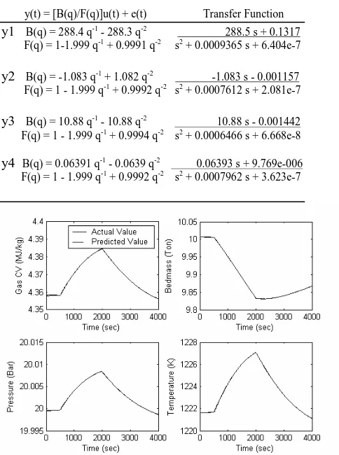
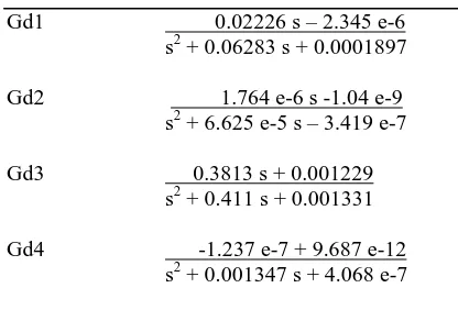
For step tests in char flow (u1) as shown in Figure 2, the numerators and denominators of the transfer functions are summarized in Table 2. Plots of actual responses and the simulated values using the identified models are shown in Figure 3. It can be seen that the models are satisfactory.

Figure 2. Profile of input and disturbance variables for step up and down of char flow (u1).

Table 2. Identified models

y(t) = [B(q)/F(q)]u(t) + e(t) Transfer Function

y1 B(q) = 288.4 q-1_{- 288.3 q}-2_{288.5 s + 0.1317}

F(q) = 1-1.999 q-1_{+ 0.9991 q}-2_s2_{+ 0.0009365 s + 6.404e-7} y2 B(q) = -1.083 q-1_{+ 1.082 q}-2_{-1.083 s - 0.001157}

F(q) = 1 - 1.999 q-1 + 0.9992 q-2 s2 + 0.0007612 s + 2.081e-7

y3 B(q) = 10.88 q-1_{- 10.88 q}-2_{10.88 s - 0.001442}

F(q) = 1 - 1.999 q-1_{+ 0.9994 q}-2_s2_{+ 0.0006466 s + 6.668e-8} y4 B(q) = 0.06391 q-1_{- 0.0639 q}-2_{0.06393 s + 9.769e-006}

F(q) = 1 - 1.999 q-1 + 0.9992 q-2 s2 + 0.0007962 s + 3.623e-7

Figure 3. Actual process outputs and the simulated values from the identified linear model

(4)

+ 10% and -10% of the corresponding steady state values of the manipulated variables at times 500 s and 2000 s. For pressure disturbance test, step up and down values are ± 0.2 bar.

Table 3. Identified transfer functions

G Transfer Function

G11 288.5 s + 0.1317

s2 + 0.0009365 s + 6.404e-7

G21 -1.083 s - 0.001157

s2 + 0.0007612 s + 2.081e-7

G31 10.88 s - 0.001442

s2 + 0.0006466 s + 6.668e-8

G41 0.06393 s + 9.769e-006

s2 + 0.0007962 s + 3.623e-7

G12 -6927 s +1.95

s2 + 0.04927 s + 6.26 e-5

G22 -0.428 s + 0.000201

s2 – 0.0003426 s – 3.039 e -8

G32 2444 s + 6.167

s2 + 0.2465 s + 0.0003653

G42 0.04664 s + 1.779 e-5

s2 + 0.001197 s + 5.86 e-7

G13 5303 s – 6.382

s2 + 0.03363 s + 4.306 e-5

G23 0.5327 s + 0.001158

s2 + 0.001245 s + 2.746 e-7

G33 1039 s – 1.618

s2 + 0.2468 s + 0.0003226

G43 -0.05418 s + 1.318 e-5

s2 + 0.0005866 s – 9.745 e-8

G14 5035 s – 1.029

s2 + 0.02632 s + 8.23 e-6

G24 -0.7753 s – 0.004223

s2 + 0.007574 s + 5.086 e-6

G34 4800 s + 0.4871

s2 + 0.3032 s + 9.41 e-5

G44 -0.005225 s – 4.671 e-5

s2 + 0.00226 s + 9.812 e-7

G15 -183.3 s + 0.05493

s2 + 0.0003089 s – 1.073 e-7

G25 0.219 s + 0.0009288

s2 + 0.001592 s + 3.119 e-7

G35 439.6 s – 0.2743

s2 + 0.0958 s + 8.924 e-5

G45 -0.02776 s – 4.475 e-5

s2 + 0.001509 s + 1.233 e-6

Gd1 0.02226 s – 2.345 e-6

s2 + 0.06283 s + 0.0001897

Gd2 1.764 e-6 s -1.04 e-9

s2 + 6.625 e-5 s – 3.419 e-7

Gd3 0.3813 s + 0.001229

s2 + 0.411 s + 0.001331

Gd4 -1.237 e-7 + 9.687 e-12

s2 + 0.001347 s + 4.068 e-7

The process model identification here is based on the simulated process operation data at 100% load case and will be used for control operability analysis of control structures given in Asmar et al. (2000), which are also based solely on 100% load.

4. GRDG ANALYSIS FOR THE ALSTOM

GASIFIER

The steady state gain matrix (based on the identified transfer functions) for the ALSTOM gasifier is presented below: ( )             − − − − − − − − − − − − = 2936 . 36 6050 . 47 2488 . 135 3584 . 30 9638 . 26 3 0737 . 3 3 1764 . 5 3 0155 . 5 4 6882 . 1 4 1626 . 2 3 9779 . 2 3185 . 830 3 2170 . 4 3 6140 . 6 3 5598 . 5 5 1193 . 5 5 2503 . 1 5 4821 . 1 4 1150 . 3 5 0565 . 2 0 e e e e e e e e e e e e e e G

From the above steady state gain matrix, the 5th

column is deleted since u5 is set to 10% of u3 in closed loop system. This left 4 degree of freedom and the matrix is now square matrix.

( )

            − − − − − − − − − = 6050 . 47 2488 . 135 3584 . 30 9638 . 26 3 1764 . 5 3 0155 . 5 4 6882 . 1 4 1626 . 2 3185 . 830 3 2170 . 4 3 6140 . 6 3 5598 . 5 5 2503 . 1 5 4821 . 1 4 1150 . 3 5 0565 . 2 0 e e e e e e e e e e e G

Based on Table 3, the steady state vector disturbance can also be calculated:

( )

            − − = 5 3813 . 2 9234 . 0 0030 . 0 0124 . 0 0 e Gd

RDGA matrix is calculated by using Equation (5):

            − − − − − − − = 4247 . 132 1588 . 163 3498 . 62 6157 . 30 3713 . 0 1560 . 0 8941 . 0 6332 . 0 3339 . 18 3807 . 40 8234 . 107 1089 . 50 9180 . 667 3579 . 343 8589 . 122 4189 . 448 β

(5)

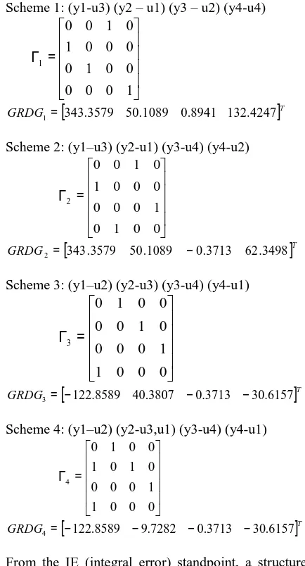
Scheme 1: (y1-u3) (y2 – u1) (y3 – u2) (y4-u4)

   

 

   

 

= Γ

1 0 0 0

0 0 1 0

0 0 0 1

0 1 0 0

1

[

]

T

GRDG₁= 343.3579 50.1089 0.8941 132.4247

Scheme 2: (y1–u3) (y2-u1) (y3-u4) (y4-u2)

   

 

   

 

= Γ

0 0 1 0

1 0 0 0

0 0 0 1

0 1 0 0

2

[

]

T

GRDG2 = 343.3579 50.1089 −0.3713 62.3498

Scheme 3: (y1–u2) (y2-u3) (y3-u4) (y4-u1)













=

Γ

0

1

0

1

0

1

0

3

[

]

T

GRDG3= −122.8589 40.3807 −0.3713 −30.6157

Scheme 4: (y1–u2) (y2-u3,u1) (y3-u4) (y4-u1)

   

 

   

 

= Γ

0 0 0 1

1 0 0 0

0 1 0 1

0 0 1 0

4

[

]

T

GRDG4= −122.8589 −9.7282 −0.3713 −30.6157

From the IE (integral error) standpoint, a structure

giving small value in

δ

_iis preferred (Chang and Yu,

1992). It is obvious that Scheme 4 is the most favourable pairing among the 4 schemes. It can also be concluded from these GRDG values that Scheme 2 would be better than Scheme 1 and Scheme 3 would be better than Scheme 2 in terms of disturbance rejection performance. Simulation results in (Asmar et al., 2000) and (Dixon and Pike, 2004) confirmed these.

Figure 4. Process response to step pressure disturbance at 100% load

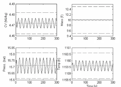
Figure 7. Process response to sinusoidal pressure disturbance at 100% load

(6)

Figure 8. Process response to sinusoidal pressure disturbance at 50% load

5. CONCLUSIONS

A systematic method for assessing the disturbance rejection performance of different control structures for the ALSTOM gasifier using GRDG is presented in this paper. The analysis is based on the transfer function model identified from the simulated process operation data based on the nonlinear simulation programme. The OE method is used in identifying process models because it can lead to models with good long range prediction (simulation) performance and, hence, accurate transfer function models. It is shown that Scheme 4 is the most favoured control structure among the 4 control structures considered. Simulation results confirm this finding. Studies in this paper also indicate that using RGA analysis is not effective in control structure selection for this benchmark process. It would be possible to find even better control structures using GRDG analysis and this is under further investigation.

ACKNOWLEDGMENT

This work was supported by Technological and Professional Skills Development Sector Project (TPSDP) – ADB Loan No.1792 – INO. This support is gratefully acknowledged.

REFERENCES

Asmar, B. N., Jones, W. E., and Wilson, J. A. (2000). A process engineering approach to the

ALSTOM gasifier problem. Proceedings of

the Institution of Mechanical Engineers Part I-Journal of Systems and Control Engineering, v. 214, no. 16, p. 441-452. Bristol, E. (1966). On a new measure of interaction

for multivariable process control. IEEE

Transaction on Automaatic Control, v. 11, no. 1, p. 133-134.

Burnham, K., Young, P., and Dixon, R. (2000). Special issue on the ALSTOM gasifier control engineering benchmark challenge.

Proceedings of the Institution of Mechanical Engineers Part I-Journal of Systems and Control Engineering, v. 214, no. 16, p. I-II.

Chang, J. W., and Yu, C. C. (1992). Relative

Disturbance Gain Array. Aiche Journal, v.

38, no. 4, p. 521-534.

Dixon, R., and Pike, A. W. (2004). Introduction to the 2nd ALSTOM benchmark challenge on

gasifier control, inControl 2004, Bath, UK.

Dixon, R., Pike, A. W., and Donne, M. S. (2000). The ALSTOM benchmark challenge on

gasifier control. Proceedings of the

Institution of Mechanical Engineers Part I-Journal of Systems and Control Engineering, v. 214, no. 16, p. 389-394.

Griffin, I. A., Schroder, P., Chipperfield, A. J., and Fleming, P. J. (2000). Multi-objective optimization approach to the ALSTOM

gasifier problem. Proceedings of the

Institution of Mechanical Engineers Part I-Journal of Systems and Control Engineering, v. 214, no. 16, p. 453-468.

Liu, G. P., Dixon, R., and Daley, S. (2000).

Multi-objective optimal-tuning

proportional-integral controller design for the ALSTOM

gasifier problem. Proceedings of the

Institution of Mechanical Engineers Part I-Journal of Systems and Control Engineering, v. 214, no. 16, p. 395-404.

Munro, N., Edmunds, J. M., Kontogiannis, E., and Impram, S. T. (2000). A sequential loop closing approach to the ALSTOM gasifies

problem. Proceedings of the Institution of

Mechanical Engineers Part I-Journal of Systems and Control Engineering, v. 214, no. 16, p. 427-439.

Rice, M. J., Rossiter, J. A., and Schuurmans, J. (2000). An advanced predictive control approach to the ALSTOM gasifier problem.

Proceedings of the Institution of Mechanical Engineers Part I-Journal of Systems and Control Engineering,v. 214, no. 16, p. 405-413.

Stanley, G., Marinogalarraga, M., and McAvoy, T. J. (1985). Shortcut Operability Analysis .1.

The Relative Disturbance Gain. Industrial &

Engineering Chemistry Process Design and Development, v. 24, no. 4, p. 1181-1188. Taylor, C. J., McCabe, A. P., Young, P. C., and

Chotai, A. (2000). Proportional-integral-plus (PIP) control of the ALSTOM gasifier

problem. Proceedings of the Institution of

Mechanical Engineers Part I-Journal of Systems and Control Engineering, v. 214,