Optimization of Group Decision Support System in
Updated Pranata Mangsa System Using Fuzzy Multi
Criteria Decision Making (FMCDM) Method
Sri Winarso Martyas Edi1), Kristoko Dwi Hartomo2), Sri Yulianto Joko Prasetyo3)
1
Fakultas Teknologi Informasi, Universitas Kristen Satya Wacana Salatiga, Jawa Tengah, Indonesia
2
Fakultas Teknologi Informasi, Universitas Kristen Satya Wacana Salatiga, Jawa Tengah, Indonesia
3
Fakultas Teknologi Informasi, Universitas Kristen Satya Wacana Salatiga, Jawa Tengah, Indonesia
Abstract
Farmers have used a natural phenomenon as an indicator of planting pattern arrangement in the form of local knowledge of pranata mangsa, however, the accuracy level of traditional prediction is frequently biased nowadays, hence requiring a model to assist agriculture department, agricultural extension workers and farmers in decision making of an effective planting pattern determination. In order to respond this matter, Fuzzy Multi Criteria Decision Making (FMCDM) and triangular fuzzy number methods with 19 sub-districts in Boyolali as land alternatives, 3 climate criteria and 3 decision makers would be applied. The alternative commodities consist of rice, corn and soybeans.
The result shows that rice is compatible in Banyudono, Mojosongo, Ngemplak and Boyolali with value of 0.3; while corn is compatible in Sambi, Teras, Sawit and Banyudono with value of 0.55; and soybean is compatible in Teras, Sawit and Sambidengan with value of 0.36. The advantage of this study is as an innovation of soft computing technology in agriculture and used as a decision making proponent.
Keywords : fuzzy multi criteria decision making, gdss,
planting pattern, pranatamangsa
1.
Introduction
The decision making matter plays significant roles in many aspects of life [1]. There are several conditions that are probably experienced by the decision maker when making any decision, namely [2] : (1) decision making in certainty, in which all alternatives are figured out, (2) decision making in some selected risk level, (3) decision making in uncertainty condition, including the alternative that is not obviously figure out.
MCDM is a method that can be used as a tool of supporting decision. Multicriteria Decision Making Methods (MCDM) refers to the process of screening, prioritizing, ranking or choosing an alternative set with criteria conditions of independent, incommensurate or conflicting [3]. MCDM is very appropriate to be implemented in all alternative cases, containing some criteria of which each has nominal value. Each criterion has quality that can be applied as comparison tool. MCDM assumed that alternative rating and quality of criteria are regarded as crips. Not all cases, however, accomplished the assumption; hence MCDM consideration is less proper and requiring some new considerations [4]. FMCDM is a decision making method considering some alternatives and criteria of a condition regarded as fuzzy [5].
The problem to be solved in this paper relates to the exploration of suitability of the proper areas for rice, corn and soybean commodities in Boyolali comprising 19 sub-districts. There are three plants that would be alternative plants, i.e. rice, corn and soybean. Criteria used as the condition of plant growth consist of temperature, rainfall and humidity. The result was supposed to gain the planting suitability pattern in sub-district areas that could be obtained in a quite prompt period by considering criteria and weights.
2.
Related Works
giving decision [6]. Regarding some literatures indicating some stages that needed to take to apply FMCDM, Cahyo and Wahyuni [5] agreed with Chou[7], Lee, Wang &Pang[8], Haarstrick and Lazarevska[9]. These four journalist conveyed similar stages to Elanchezhian, Ramnath and Kesavan[10].
Those four articles conveyed stages of accomplishing FMCDM that supported each other. By adapting those four articles, the three stages of FMCDM process were required, i.e. problem representation, evaluation of fuzzy sets of every decision alternatives, and selection of the optimum alternatives.
3.
Theoretical Framework
Each plant has different growth conditions. Based on the 3 plants to be planted, rice can grow well in tropical and moist areas. The fine rainfall distribution for 4 months and the average of 200 mm per month or more, around 1500 – 2000 mm per year. The fine temperature for rice growth is 23C. The appropriate altitude for rice is around 0 – 1500 m dpl. The fine land for rice growth is rice field land containing sand, dust and clay segments in certain ratio as well as requiring sufficient amount of water. Rice can grow well in the soil with the top layer of 18 – 22 cm thick and pH of 4 -7 [11].
Unlike rice, the disposed of climate for corn is mostly the temperate climate to humid subtropical climate. Corn can grow in the area with an altitude of 0 – 50C LU up to 0 – 40LS. In non-irrigated land, the plant growth requires ideal rainfall which is around 85 – 200 mm/ month and should be evenly spread. In the phase of flowering and grain-filling, corn needs to get enough water. Corn should be planted in the early season, just before the dry season. The corn growth requires sunlight. The growth of shaded corn would be hampered as well as the seed crops were not good enough, and the fruit could not grow properly. The disposed temperature of corn is around 21 - 34C, in which the ideal plant growth requires optimum temperature around 23 - 27C. The proper temperature of corn seed sprouting process is around 30C. Corn harvest in the dry season would be better than wet season since influencing the ripening time and crops drying [12].
Meanwhile, soybean mostly grows in tropical and subtropical areas. Whether the climate is appropriate for corn, it can be used as a barometer of proper climate of soybean. The durability of soybean is better than corn indeed. The dry climate is more
preferred to moist climate for soybean. Soybean can grow well in areas with rainfall of 100 – 400 mm/ months. Meanwhile, in order to get an optimal result, soybean requires rainfall of 100 – 200 mm/ month. The disposed temperature of soybean is around 21 – 34C, however, the optimal temperature for soybean growth is around 23 – 27C. The proper temperature of soybean seed sprouting process is around 30C. Soybean harvest in a dry season would be better than wet season since influencing the seed ripening time and the yield drying [13].
This study employed Fuzzy MCDM method. Multi Criteria Decision Making is a method for assisting the decision making towards some decision alternatives which should be taken by considering some criteria [14]. A problem probably emerged in case there was uncertainty within the importance weights of each criterion and the degree of suitability of each alternative to each criterion [15]. The assessment given by the decision maker is conducted through qualitative and presented using linguistic way [16].
In Javanese culture, there is a science of weather and climate forecast which is called pranatamangsa. Pranatamangsa comes from the words ‘pranata’ which mean procedure and ‘mangsa’ which means season [17]. This culture is not only found in Java, but also in Bali which is called as Wariga as well as in Sunda that is called as Kala. Pranatamangsa that exists all along, mostly used theory based on socially economical of agriculture [18], however, along with the development of technology, the studies of pranatamangsa have been conducted by engaging the other fields of study, for instance, the studies conducted by Hartomo, Sediyono, Yulianto and Simanjutak [19] with an issue of pranatamangsa combined with Local Knowledge and Agro-meteorology using Fuzzy Logic to determine plant pattern as the improvement of the previous studies with Agro-meteorology-based using LVQ, MAP ALOV [20].
4.
Research Method
T(x). For instance, the rating for weight of Significant Variable of a criterion defined as: T(significant) = {VERY LOW, LOW, FAIR, HIGH, VERY HIGH}. After the determination of this set of rating was conducted, the membership function of each rating should be determined afterward. The triangle function is commonly used for it. For instance, Wt is the weight of Ct criterion; and Sit is fuzzy rating for the degree of suitability of Ai decision alternative and Ct criterion; as well as Fi is fuzzy suitability index of Ai alternative representing the degree of suitability of decision alternatives and decision criteria obtained from the aggregation result of Sit and Wt.
The second activity are evaluating the criteria weights and the degree of suitability of each alternative and its criteria.
The third activity is aggregating the criteria weights and the degree of suitability of each alternative and its criteria. There are some methods which can be used to aggregate the decision results of the decision makers, such as: mean, median, max, min, and combine operator. From those methods, mean is the most frequently used. Mean is the operator used for the adding and multiplication of fuzzy.
By using mean, Fi is formulated as:
Ft= 1
k [(St1⊗ W1)⊕(St2⊗ W2)⊕∧⊕(Stk⊗ Wk) ] (1)
By substituting Sit and Wt with triangular fuzzy number, that is Sit = (oit, pit, qit); and Wit = at,bt,ct); Ft can be approached as:
Fi ≅ Yi, Qi, Zi (2)
With
Yi= 1
k ∑ (oit,ai) k
t=1 (3)
Qi= 1
k ∑kt=1 pit,bi (4)
Zi= 1
k ∑kt=1 qit,ci (5)
i=1,2,3,…,n.
The fourth activity is prioritizing the decision alternatives based on aggregation result. The priority of aggregation result was required regarding the ranking process of decision alternatives.
In order to determine the order of each alternative, the following equation can be engaged:
Si= ∑nj=1rij (6)
A method of total integral value can be used. For instance, F is a triangular fuzzy number, F = (a, b, c), the total integral value can be formulated as follows:
ITα(F)= 1
2 αc+b+ 1- α a (7)
α value is the optimism index representing the degree of optimism of decision makers (0≤α≤1).
In case α value is greater, indicating that the degree of optimism is greater, as well.
Choosing the decision alternatives with the highest priority as the optimum alternative. The greater the Fi value indicates the biggest suitability of decision alternatives of decision criteria and this value would be the goal.
5.
Architectural Design
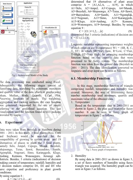
Architectural model that is used in this study can be seen in figure 1. The study was conducted in 5 stages.
In stage 1, The Temperature, Rainfall and Humidity during 2001 – 2011 data of Boyolali that can be seen in boyolali in numbers collected, and pre-processing data was conducted afterwards.
Stage 2 comprises weighting process and value aggregation of the data result which has been conducted as well as the information of plant growth condition and input result from some plant experts.
Stage 3 comprises the process of sorting plant suitability toward an area.
Stage 4 comprises the process of searching the optimism value of the ranking result which has been conducted in the previous stage.
Fig 1. Architectural Model of the Study
The data processing was conducted using Excel. Subsequently, the following stages consist of classifying data, searching the minimum, maximum and quartile value of the data, charts or graphs using Mean, Median, Mode, Quartile, CCart, Plot, Piecewise functions of maple. The weighting, aggregation and ranking sections, the own function was generated, supported by the use of maple referring to the predefined equation. The last visualization used the function found in GUI package provided by maple.
6.
Experiment
Data were taken from Boyolali in Numbers during 2001 – 2011. In this study, 3 food plants (Rice, Corn and Soybean) would be searched for the compatibility of growing in certain areas and 19 alternatives of places to plant the 3 food plants, namely Selo, Ampel, Cepogo, Musuk, Boyolali, Mojosongo, Teras, Sawit, Banyudono, Sambi, Ngemplak, Nogosari, Simo, Karanggede, Klego, Andong, Kemusu, Wonosegoro, Juwangi sub-districts. Besides, 3 criteria (indications) of decision making consist of temperature; rainfall; humidity and 3 decision makers comprise D1, D2 and D3 who have expertise and proficiency in plant growth conditions.
By using equation 8 :
A = {Ai | i=1,2,…,n} (8)
determined that 19 alternatives of plant areas comprise A = {A1,A2,A, ..., A19}, in which A1=Selo, A2=Ampel, A3=Cepogo, A4=Musuk, A5=Boyolali, A6=Mojosongo, A7=Teras, A8=Sawit,
A9=Banyudono, A10=Sambi, A11=Ngemplak,
A12=Nogosari, A13=Simo, A14=Karanggede,
A15=Klego, A16=Andong, A17= Kemusu,
A18=Wonosegoro, A19=Juwangi. Besides, by using equation 9 :
C = {Ct | t=1,2,…,k} (9)
determined that 3 criteria (indications) of decision are C ={C1,C2,C3}
Linguistic variables representing importance weights of each criterion are T(importance) W1 = {SR, R, C, T, ST} in which SR=Very Low, R=Low, C=Fair, T=High, ST=Very High} by arranging membership function based on the expert’s data that were processed to be fuzzy system. The membership function was taken from the ground data (Boyolali in 2001 – 2011). The data identification converted to linguistic and crisp input can be seen as follows.
6.1. Membership Function
In this stage, membership function of triangle comprising rainfall, temperature and humidity was created. Moreover, the way of determining fuzzy number membership used minimum, quartile and maximum value of the obtained data.
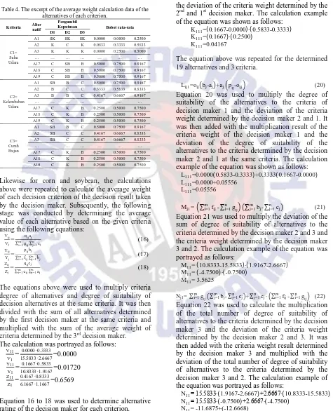
1. Temperature
Based on the temperature data in 2001-2011 as shown in figure 2, the plan used triangular fuzzy number. It can be seen in fuzzy graph of temperature in figure 2 as follows.
Fig 2. Fuzzy graph of temperature.
2. Humidity
Fig 3. Fuzzy graph of temperature
3. Rainfall
By using data in 2001-2011 as shown in figure 4, a set of the fuzzy number of rainfall using fuzzy triangle was acquired. The fuzzy graph of rainfall can be seen in figure 4 as follows.
Fig 4. Fuzzy graph of rainfall
6.2. Degree of Suitability
Degree of suitability of alternatives and decision criteria comprise: T(suitability) S= {SK, K, C, B, SB}, in which SK = Very Little; K = Less; C = Fair; B = Good; SB = Very Good; in which each of them was represented with triangular fuzzy number as follows:
SK = (0.00, 0.00, 0.25) K = (0.00, 0.25, 0.50) C = (0.25, 0.50, 0.75) B = (0.50, 0.75, 1.00) SB = (0.75, 1.00, 1.00)
In the following stage, the decision makers gave weight for every criterion of each food plant and rating for the alternatives of each criterion, as well. The average weight of each criterion for the decision makers of each planting was accomplished by using equations of:
aj=∑kt=1ajt
k (10)
bj=∑ bjt
k t=1
k (11)
cj= ∑ cjt
k t=1
k (12)
The equations above were used to sum crisp value of the decision result determined by the decision maker
based on the value of importance weights of each criterion. It was then divided with the total of decision makers, for instance, the calculation of the importance weight average of rice; in which the calculation can be seen as follows:
a1=0.50+0.25+0.50
3 =0.4167
b1=0.75+0.50+0.75
3 =0.6667
c1=
0.10+0.75+0.10
3 =0.9167
Thus, the whole determination of the importance weight average of rice, corn, and soybean can be seen in table 1, 2 and 3 as follows:
Table 1. Weight of criteria of rice planting decision maker.
Kriteria
Pengambil
Keputusan Crisp
D1 D2 D3
C1 = Suhu Udara T C T 0.4167, 0.6667, 0.9167 C2 = Kelembaban T T T 0.5000, 0.7500, 1.0000 C3 = Curah Hujan R C T 0.2500, 0.5000, 0.7500
Table 2. Weight of criteria of corn planting decision maker.
Kriteria
Pengambil
Keputusan Crisp
D1 D2 D3
C1 = Suhu Udara T ST T 0.5833, 0.8333, 1.0000 C2 = Kelembaban T ST T 0.5833, 0.8333, 1.0000 C3 = Curah Hujan T ST T 0.5833, 0.8333, 1.0000
Table 3. Weight of criteria of soybean planting decision maker.
Kriteria
Pengambil
Keputusan Crisp
D1 D2 D3
C1 = Suhu Udara T C C 0.3333, 0.5833, 0.8333 C2 = Kelembaban T C T 0.4167, 0.6667, 0.9167 C3 = Curah Hujan T C T 0.4167, 0.6667, 0.9167
After the decision maker inputted the weights, the average weight of the alternatives of each criterion of rice, corn and soybean referred to equations of:
eij= ∑ aijt
k t=1
k (13)
fij=∑ fijt
k t=1
k (14)
gij=∑ gijt
k t=1
k (15)
The equations above were used to add up crisp value of predefined decision of the decision maker based on linguistic value of the degree of suitability of the alternatives and each decision criterion. It was then divided with the total of decision makers.
The calculation of alternative Selo with criterion 1-Temperature was figured out as follows:
e11=0.00+0.00+0.00
3 =0.0000
f11=0.00+0.00+0.00
3 =0.0000
g11=0.25+0.25+0.25
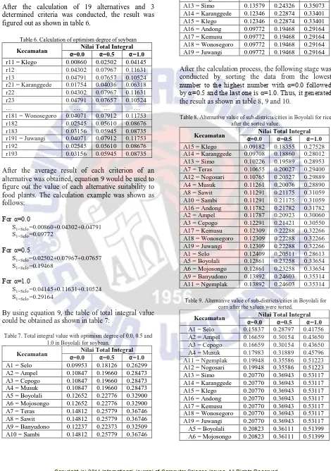
The calculations above were applied to 19 sub-districts alternatives with 3 determined criteria. The excerpt of rice calculation data was portrayed in Table 4.
Table 4. The excerpt of the average weight calculation data of the alternatives of each criterion. of each decision criterion of the decision result taken by the decision maker. Subsequently, the following stage was conducted by determining the average decision alternatives at the same criteria. It was then divided with the sum of all alternatives determined by the first decision maker at the same criteria and multiplied with the sum of the average weight of criteria determined by the 3rd decision maker.
The calculation was portrayed as follows:
V11 rating of the decision maker for each criterion.
Kij1= pij-oij bj-aj (19)
Equation 19 was used to seek the deviation of the average weight of the degree of suitability for the 2nd and 1st decision maker. It was then multiplied with the deviation of the criteria weight determined by the 2nd and 1st decision maker. The calculation example of the equation was shown as follows:
K111=(0.1667-0.0000)∙(0.5833-0.3333) K111=(0.1667)∙(0.2500)
K111=0.04167
The equation above was repeated for the determined 19 alternatives and 3 criteria.
Lij1=oij bj-aj +aj pij-oij (20) Equation 20 was used to multiply the degree of suitability of the alternatives to the criteria of decision maker 1 and the deviation of the criteria weight determined by the decision maker 2 and 1. It was then added with the multiplication result of the criteria weight of the decision maker 1 and the deviation of the degree of suitability of the alternatives to the criteria determined by the decision maker 2 and 1 at the same criteria. The calculation example of the equation was shown as follows:
L111=0.0000(0.5833-0.3333)+0.3333(0.1667-0.0000) L111=0.0000+0.05556 Equation 21 was used to multiply the deviation of the sum of degree of suitability of alternatives to the criteria determined by the decision maker 2 and 3 and the criteria weight determined by the decision maker 3 and 2. The calculation example of the equation was portrayed as follows:
M11=(10.8333-15.5833)∙(1.9167-2.6667) Equation 22 was used to calculate the multiplication of the total number of degree of suitability of alternatives to the criteria determined by the decision maker 3 and the deviation of the criteria weight determined by the decision maker 2 and 3. It was then added with the criteria weight result determined by the decision maker 3 and multiplied with the deviation of the total number of degree ofsuitability of alternatives to the criteria determined by the decision maker 3 and 2. The calculation example of the equation was portrayed as follows:
N11= 15.5833∙(1.9167-2.6667)+2.6667∙(10.8333-15.5833) N11= 15.5833∙(-0.7500)+2.6667∙(-4.7500)
N11= -11.6875+(-12.6668)
Kij2= pij-qij bj-cj (23) Equation 23 was used to seek the deviation of the average weight of degree of suitability for the 2nd and 3rd decision maker. It was then multiplied with the deviation of the criteria weight determined by the 2nd and 3rd decision maker. The calculation example of the equation was portrayed as follows:
K112=(0.1667-0.4167)∙(0.5833-0.8333) K112=(-0.2500)∙(-0.2500)
K112=0.0625
Lij2=qij bj-cj +cj pij-qij (24) Equation 24 was used to multiply the degree of suitability of alternatives to the criteria of the decision maker 3 and multiplied with the deviation of the criteria weight determined by the decision maker 2 and 3. It was then added with the multiplication result of the criteria weight of the decision maker 3 and the deviation of degree of suitability of alternatives to the criteria determined by the decision maker 2 and 3 at the same criteria. The calculation example of the equation was portrayed as follows:
L112=0.4167∙(0.5833-0.8333)+0.8333∙(0.1667-0.4167) L112=-0.1042+(-0.2084)
L112=-0.3126
Mj2= ∑mi=1fij-∑ni=1eij ∑mj=1bj-∑nj=1aj (25) Equation 25 was used to multiply the deviation of the sum of the degree of suitability of alternatives to the criteria determined by the decision maker 2 and 1 and the criteria weight determined by the decision maker 2 and 1. The calculation example of the equation was portrayed as follows:
M12=(10.8333-6.1667)∙(1.9167-1.1667)
M12=(4.6666)∙(0.7500)
M12= 3.49995
Nj2= ∑m eij
i=1 ∑mj=1bj-∑nj=1aj +∑j=1n aj ∑mi=1fij-∑ni=1eij (26) Equation 26 was used to calculate the multiplication of the total number of degree of suitability of alternatives to the criteria determined by the decision maker 1 and the deviation of the criteria weight determined by the decision maker 2 and 1. It was then added with the result of criteria weight determined by the decision maker 1 and multiplied with the deviation of the total number of degree of suitability of alternatives to the criteria determined by the decision maker 2 and 1. The calculation example of the equation was portrayed as follows:
N12= 6.1667∙(1.9167-1.1667)+1.1667∙(10.8333-6.1667) N12= 6.1667∙(0.7500)+1.1667∙(4.6666)
N12= 4.6250+5.4445
N12= 10.069
The calculation using equation 16 to 26 was repeated for the determined 19 Alternatives and 3 Criteria. The
calculation of equation 13 – 26 was also conducted to corn and rice. Thus, the result was generated as in table 5.
Table 5. The excerpt of calculation data of soybean.
⁄ ⁄ ⁄ suitability of alternatives of planting medium for rice, corn and soybean in Boyolali areas would be obtained.
6.3. Alternative Selection Using Total
Integral Method
IT0(F)=0.041445
After the calculation of 19 alternatives and 3 determined criteria was conducted, the result was figured out as shown in table 6.
Table 6. Calculation of optimism degree of soybean
Kecamatan Nilai Total Integral
α=0.0 α=0.5 α=1.0 r11 = Klego 0.00860 0.02502 0.04145
r12 0.04302 0.07967 0.11631
r13 0.04791 0.07657 0.10524
r21 = Karanggede 0.01754 0.04036 0.06318
r22 0.04302 0.07967 0.11631
r23 0.04791 0.07657 0.10524
… … … …
r181 = Wonosegoro 0.04071 0.07912 0.11753
r182 0.02545 0.05610 0.08676
r183 0.03156 0.05945 0.08735
r191 = Juwangi 0.04071 0.07912 0.11753
r192 0.02545 0.05610 0.08676
r193 0.03156 0.05945 0.08735
After the average result of each criterion of an alternative was obtained, equation 9 would be used to figure out the value of each alternative suitability to food plants. The calculation example was shown as follows:
For α=0.0
S1=Selo=0.00860+0.04302+0.04791
S1=Selo=0.09772
For α=0.5
S1=Selo=0.02502+0.07967+0.07657
S1=Selo=0.19468
For α=1.0
S1=Selo=0.04145+0.11631+0.10524 S1=Selo=0.29164
By using equation 9, the table of total integral value could be obtained as shown in table 7:
Table 7. Total integral value with optimism degree of 0.0, 0.5 and 1.0 in Boyolali for soybean.
Kecamatan α Nilai Total Integral =0.0 α=0.5 α=1.0 A1 = Selo 0.09953 0.18126 0.26299 A2 = Ampel 0.10847 0.19660 0.28473 A3 = Cepogo 0.10847 0.19660 0.28473 A4 = Musuk 0.10847 0.19660 0.28473 A5 = Boyolali 0.12652 0.22776 0.32900 A6 = Mojosongo 0.12652 0.22776 0.32900 A7 = Teras 0.14812 0.25779 0.36746 A8 = Sawit 0.14812 0.25779 0.36746 A9 = Banyudono 0.12237 0.22373 0.32509 A10 = Sambi 0.14812 0.25779 0.36746
A11 = Ngemplak 0.11358 0.21195 0.31031 A12 = Nogosari 0.13116 0.23551 0.33986 A13 = Simo 0.13579 0.24326 0.35073 A14 = Karanggede 0.12346 0.22874 0.33401 A15 = Klego 0.12346 0.22874 0.33401 A16 = Andong 0.09772 0.19468 0.29164 A17 = Kemusu 0.09772 0.19468 0.29164 A18 = Wonosegoro 0.09772 0.19468 0.29164 A19 = Juwangi 0.09772 0.19468 0.29164
After the calculation process, the following stage was conducted by sorting the data from the lowest number to the highest number with α=0.0 followed by α=0.5 and the last one is α=1.0. Thus, it generated the result as shown in table 8, 9 and 10.
Table 8. Alternative value of sub-districts/cities in Boyolali for rice after the sorted value.
Kecamatan Nilai Total Integral
α=0.0 α=0.5 α=1.0 A15 = Klego 0.09182 0.18355 0.27528 A14 = Karanggede 0.09708 0.18860 0.28012 A13 = Simo 0.10226 0.19589 0.28953 A7 = Teras 0.10655 0.20027 0.29400 A12 = Nogosari 0.10765 0.20327 0.29889 A4 = Musuk 0.11261 0.20076 0.28890 A8 = Sawit 0.11291 0.21175 0.31059 A10 = Sambi 0.11291 0.21175 0.31059 A16 = Andong 0.11782 0.21782 0.31782 A2 = Ampel 0.11787 0.20923 0.30060 A3 = Cepogo 0.12291 0.21421 0.30550 A17 = Kemusu 0.12309 0.22288 0.32266 A18 = Wonosegoro 0.12309 0.22288 0.32266 A19 = Juwangi 0.12309 0.22288 0.32266
A1 = Selo 0.12409 0.20511 0.28613
A5 = Boyolali 0.12861 0.23258 0.33654 A6 = Mojosongo 0.12861 0.23258 0.33654 A9 = Banyudono 0.13892 0.24603 0.35314 A11 = Ngemplak 0.13892 0.24603 0.35314
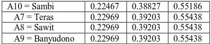
Table 9. Alternative value of sub-districts/cities in Boyolali for corn after the values were sorted.
Kecamatan Nilai Total Integral
A10 = Sambi 0.22467 0.38827 0.55186 A7 = Teras 0.22969 0.39203 0.55438 A8 = Sawit 0.22969 0.39203 0.55438 A9 = Banyudono 0.22969 0.39203 0.55438
Table 10. Alternative value of sub-districts/cities in Boyolali for soybean after the values were sorted.
Kecamatan α Nilai Total Integral =0.0 α=0.5 α=1.0 A16 = Andong 0.09772 0.19468 0.29164 A17 = Kemusu 0.09772 0.19468 0.29164 A18 = Wonosegoro 0.09772 0.19468 0.29164 A19 = Juwangi 0.09772 0.19468 0.29164 A14 = Karanggede 0.12346 0.22874 0.33401 A15 = Klego 0.12346 0.22874 0.33401
The bigger the α value, the higher the plant suitability level for those areas was. Furthermore, the smaller the value or in the top order, the lower the plant suitability level for those areas was. Thus, the most compatible areas for rice commodity comprise
Ngemplak, Sawit, Teras Sambi, Juwangi,
Wonosegoro, and incompatible for Selo, Ampel, Cepogo, Musuk. Besides, the most compatible areas for corn commodity comprise Banyudono, Sawit,
Teras, Sambi, Juwangi, Wonosegoro, and
incompatible for Selo, Ampel, Cepogo, Musuk, Ngemplak. Otherwise, the most compatible areas for soybean commodity comprise Sambi, Sawit, Teras, Simo, Nogosari and incompatible for Selo, Andong, Kemusu, Wonosegoro, Juwangi.
7.
Conclusion and Future Work
From the result of the study above, it can be concluded that the most appropriate areas for rice commodity consist of Ngemplak, Sawit, Teras Sambi, Juwangi, Wonosegoro. Otherwise, the inappropriate areas comprise Selo, Ampel, Cepogo, Musuk. Besides, the most appropriate areas for corn commodity consist of Banyudono, Sawit, Teras, Sambi, Juwangi, Wonosegoro. Otherwise, the inappropriate areas comprise Selo, Ampel, Cepogo, Musuk, Ngemplak. Moreover, the most appropriate
areas for soybean commodity consist of Sambi, Sawit, Teras, Simo, Nogosari. Otherwise, the inappropriate areas comprise Selo, Andong, Kemusu, Wonosegoro, Juwangi.
As a suggestion for the improvement of future study, the data providing is supposed to be better. Thus, the calculation result should be visualized in form of map.
References
[1] Kusumadewi, Sri, Penetuan Lokasi Pemancar Televisi Menggunakan Fuzzy Multi Criteria Decision Making, Media Informatika Vol. 2 Desember 2004 ISSN : 0854-4743, 2004.
[2] Kusrini, Konsep dan Aplikasi Sistem Pendukung Keputusan, Andi Yogyakarta, Yogyakarta , 2007. [3] Wang S., Lee C., Tzeng G., Fuzzy Multi Criteria
Decision Making For Evaluating The Performance of Mutual Funds, 2005.
[4] Rosnelly, Rika, Retantyo Wardoyo., Penerapan Fuzzy Multi Criteria Decision Making(FMCDM)Untuk Diagnosis Penyakit Tropis,SemNas IF ISSN : 197-2328, UPN Veteran - Yogyakarta, 2011.
[5] Nur Cahyo, Winda, Wahyuni R., Implementasi Fuzzy Multicriteria Decision Making untuk Menentukan Peringkat Calon Penerima Beasiswa, Seminar Nasional Electrical, Informatics, and It’s Education, 2009.
[6] Fan,S., Shen, Q., Luo, X., and Xue, X, Comparative Study of Traditional and Group Decision Support-Supported Value Management Workshops.J. Manage Eng. ISSN:0742-597X, 29(4), 2013, 345-354. [7] C.C, Chou, A Fuzzy MCDM method for solving
marine transshipment container port selection problems, Applied Mathematics and Computation 186, 2007, 435-444.
[8] Lee, Wei-Hsuan, Chien Hua Wang, Chin-Tzong Pang, Evaluating Service Quality of Online Auction by Fuzzy MCDM, 2005, 841-852
[9] Haarestrick, Andreas and Ana Lazarevska, Multi Criteria Decision Making MCDM-A Conceptual Approach To Optimal Landfill Monitoring, Third International Workshop “Hydro-Physico-Mechanics of Landfills”, Braunschweig, Germany, March 2009. [10] Elanchezhian, C, B. Vijaya Ramnath, R. Kesavan,
Vendor Evaluating Using Multi Criteria Decision Making Technique, IJCA(0975-8887), Vol 5-No, 9 August 2010.
[11] Balai Besar Pengkajian dan Pengembangan Teknologi Pertanian, Teknologi Budidaya Padi, Bogor, Agro Inovasi, 2008.
[12] Purwono dan Hartono, Bertanam Jagung Unggul, Jakarta, Penebar Swadaya, 2007.
[13] Pitojo, Setijo, Seri Penangkaran: Benih Kedelai, Yogyakarta, Penerbit Kanisius, 2003.
Information Technology & Decision Making, Vol. 4 No.2, 2005, 277-296.
[15] Kusumadewi, Sri, Guswaludin Idham, 2005, Fuzzy Multi-Criteria Decision Making, Media Informatika ISSN : 0854-4743, Vol. 3 No.1, Juni 2005, 25-38, [16] Zadeh, L.A., The Concept Of A Linguistic Variable
And Its Application To Approximate Reasoning, Information Sciences,1975.
[17] Daldjoeni, N, Pranatamangsa, the Javanese Agricultural calendar-Its bioclimatological and sociocultural function in developing rural life, Environmentalist 1573-2991, Vol 4, Issue 7 Supplement, 1984, 15-18.
[18] Singgih, Doddy S., Metode Analisis Fungsi Lahan dalam Perspektif Sosial Pedesaan, Jurnal Masyarakat Budaya dan Politik, Th.XII No.3, 1999, 1-8. [19] Hartomo, Kristoko Dwi, Sediyono, Eko, Yulianto, Sri
dan Simanjutak, Bistok H, Updated Pranata Mangsa: Recombination of Local Knowledge and Agro Meteorology using Fuzzy Logic for Determining Planting Pattern, IJCSI, , Vol. 9. Issue 6, No. 2, November 2012, 367-372.
[20] Simanjutak, Bistok H, Hartomo, Kristoko Dwi, Yulianto, Sri, Penyusunan Model Pranatamangsa Baru Berbasis Agrometeorologi dengan Menggunakan LVQ (Learning Vector Quantization) dan MAP ALOV untuk perencanaan Pola Tanam Efektif, Laporan Akhir Hibah Bersaing Tahun-1, Salatiga : Universitas Kristen Satya Wacana, 2010.
Winarso Sri, Received is B.Sc. at Informatics Engineering from
the Satya Wacana Christian University Salatiga Indonesia. Candidate master degree at Information System at Faculty of Information Technology from the Satya Wacana Christian University Salatiga Indonesia. He is currently a lecturer in the Informatics Engineering Department, Faculty of Information Technology, Satya Wacana Christian University Salatiga Indonesia. His current research interests include web engineering, GIS, simulation and modeling, multimedia and their applications.
Hartomo Kristoko, Received is B.Sc. at Informatics Engineering
from the Duta Wacana Christian University Yogyakarta Indonesia. Received is Master degree at Computer Science at Faculty of Mathematics and Natural Sciences from the Gadjah Mada University Yogyakarta Indonesia.He is student Doctoral Program Computer Science at Faculty of Mathematics and Natural Sciences from the Gadjah Mada University Yogyakarta Indonesia. He is currently a lecturer in the Informatic Engineering Department, Faculty of Information Technology, Satya Wacana Christian University Salatiga Indonesia. His current research interests include spatial Modeling, GIS, database, data mining and their applications.
Yulianto Sri, Received is B.Sc. at Biology from the Duta Wacana
Christian University Yogyakarta Indonesia in 1995. Received is Master degree at Computer Science at Faculty of Mathematics and Natural Sciences from the Gadjah Mada University Yogyakarta Indonesia in 2002.He is Doctoral at Program Computer Science at