in PROBABILITY
WIENER SOCCER AND ITS GENERALIZATION
YULIY BARYSHNIKOV
Department of Mathematics, University of Osnabr¨uck D-49069 Osnabr¨uck, Germany.
email: [email protected]
submitted March 6, 1997;revised November 17, 1997 AMS 1991 Subject classification: 60J35 (60J65)
Wiener Process, Brownian Motion.
Abstract
The trajectory of the ball in a soccer game is modelled by the Brownian motion on a cylinder, subject to elastic reflections at the boundary points (as proposed in [KPY]). The score is then the number of windings of the trajectory around the cylinder. We consider a generalization of this model to higher genus, prove asymptotic normality of the score and derive the covariance matrix. Further, we investigate the inverse problem: to what extent the underlying geometry can be reconstructed from the asymptotic score.
0
Introduction
0.1 LetD⊂R2be the soccer field, i.e. a rectangular area with two segmentsI1, I2 marked
on two opposite sides of it, of equal length and centered at the middle of the sides. The movement of the ball is described by the trajectory of the plane Brownian motion subject to reflections at the boundary points (we neglect the event of hitting the corner as being of zero measure).
This model was proposed by Kozlov, Pitman and Yor [KPY] as a realistic description of the soccer game. They, however, investigated a far less realistic model with the field described by a half-planeℜz >0 with goalposts on the real axis.
The score, according to [3], is defined as follows. Gluing together two copies ofD along the segments I1,2 one obtains a (topological) cylinder ¯D. Choose a system of short paths on ¯D
(which associates to each point a path joining it to a base pointp0 on the cylinder so that
the lengths of the paths are bounded). Ifγ: [0, T]→D is a trajectory of the ball, then one can lift it to ¯D and close it by joining its endpoints to p0. The score Sc(T) is the winding of
the resulting closed curve around the cylinder. In other words, score represents an element of H1( ¯D,Z)∼=Z. We are interested in the asymptotic behavior of the score. It is clear that the
ambiguity of the short paths system contributes just a bounded term to the score.
0.2 The main result of [3] is that the score normed by√logT has asymptotically symmetric exponential distribution with the variance proportional to the ratio of certain elliptic integrals associated with the goalposts positions on the real line. Regarding the realistic model described
in the beginning, the authors noted that the score in this case is asymptotically Gaussian with variance growing as T (which follows quite easily from Kozlov’s results [3]) but refer to difficulties of finding the expression for variance.
The log in this theorem is typical for wandering on the complex plane (see [6] for example) and reflects the growth of the local time at zero of the Bessel process of order 2. The score in this model is the normal one with the variance exponentially distributed.
0.3 In this paper we will address the following model generalising the Wiener soccer. Let D⊂R2be a topological disk bounded by a Jordan curve ∂D,g a smooth Riemannian metric
defined in an open neighborhood ofDand{Ii}i=0,...,N a collection of nonintersecting (closed)
arcs in∂D. Gluing two copies ofDalong the arcsIione obtains a topological 2-sphere ¯Dwith
N + 1 holes. We represent the first homology group of ¯D as the factorspace H =ZN+1/(e)
where e = (1, . . . ,1). This space is generated by the cycles corresponding to the coherently oriented circumferences of the (N + 1) holes of ¯D. Fix once and forever a system of short paths in ¯D. This given, one can associate to any continuous curveγ: [0, T]→D¯ an element ofH1( ¯D,Z)∼=ZN defined up to a bounded term depending on the short paths system.
Let γ(t), t ∈ [0, T] be the Brownian motion on ¯D associated to the metricg and subject to elastic reflections at∂D¯ (we address the question how to define precisely the Brownian motion in ¯D in the next section).
Definition 0.1 We denote by Sc(T)the random element ofH1( ¯D,Z)obtained by joining the
ends of the Bronian motion γ: [0, T]→D¯ to the basepoint using the short paths system .
0.5 We are interested in the asymptotic behavior of the score. The variance of Sc(T) grows linearly in T and the expectation is bounded, so the correct scaling is Sc(T)/√T. The con-tribution of the change of the basepoint and of the short paths system to Sc(T) is bounded and therefore negligible in the scaled score. The scaled score is by definition an element of HR=H⊗R∼=RN+1/(e).
In Section 2 we investigate the asymptotics of the score. Using some general central limit theorems for martingales with bounded quadratic variations we prove the convergence of the scaled score Sc(T)/√T to a Gaussian vector inRN and determine its covariance matrix. This
covariant matrix is given by a certain quadratic form which can be given a ‘physical meaning’ as the energy loss for a conducting plate.
0.6 Further, in Section 3, we investigate the related inverseproblem. It was, actually, first posed in [1] in the context of the conducting plates mentioned above and can be formulated as follows: assume that only the asymptotical behavior of the score is known; is it possible then to reconstruct the original data (D, g,{Ii})? There is, certainly, a large group acting on the data which preserves the only observable thing, the covariance matrix (or the energy loss form): the data (hD, h∗g,{hIi}) will give the same matrix for any diffeomorphismh. One can therefore reduce the problem to the case with fixed D and g (say, the unit circle with the standard metrics). The group of diffeomorphisms preservingDandgis now three-dimensional, and the variable parameters are 2N+ 2 endpoints of the intervalsI.
We address this inverse problem in Section 3. It turns out that it can be reduced to the Shottky problem for hyperelliptic curves (solved by Mumford [5]) and thence settled completely. I would like to mention in this connection the paper [7] where an inverse problem of similar spirit has been addressed.
1
Brownian Motion in
D
¯
1.1 We start with the precise construction of the Brownian motion on the manifold with boundary ¯D. The boundary ofD consists ofN+ 1 arcsIi interlaced withN+ 1 other arcs;
we will denote them by I′
i and number them so that Ii′ lies between Ii and Ii+1; addition
in subscripts henceforth is always understood modulo (N+ 1). Let D1, D2 be two copies of
D. The (N+ 1)-holed sphere ¯D is the factor space obtained upon identification of the ‘same’ points inIi’s. The lift of the metricg fromD1,2 defines a metric on an open dense subset of
¯
D which we will refer to asgagain.
1.2 To define the Brownian motion with elastic reflections at the boundary points in the topological manifold ¯Dwe use the standard trick describing Brownian motions under conformal maps [4].
Specifically, let f : U → D be a continuous one-to-one mapping of the upper half of the complex planeU ={ℜ(·)≥0} ⊂C¯ to D which is smooth in the interior of U and takes the
conformal class of the standard metric onC(given by dx2+dy2) to that of g. Such a map
exists by theorems of Riemann and Koebe.
Let the segmentsJi = [ai, bi]∈∂U =RP1be the preimages of the arcsIi ⊂∂Dunderf (one
of these segments can contain the infinity). Define ¯S to be the Riemann sphere ¯Cwith slits
made along the intervalsJ′
i = (bi, ai+1), i= 0, . . . , N. This surface is topologically a 2-sphere
withN+ 1 holes. The mapf :U →D defined on the upper half of this holed sphere can be extended to a map ¯f : ¯S → D¯ in an obvious way. The resulting map is a homeomorphism which is smooth outside the real lineRP1.
1.3 At this stage we could already define the Brownian motion on ¯D with elastic reflections at boundary as the image under ¯f of the Brownian motion on ¯S with elastic reflections at the points of intervalsJ′
i. Changing the clock of this Brownian motion would result in a ¯D-valued
Markov process with continuous trajectories such that the generator of the corresponding semigroup is ∆g (the Laplacian ing metric) in the interiority of ¯D.
We make, however one step further in view of some applications to follow and describe the Brownian motion on ¯S itself as the projection of a Brownian motion on an adequate twofold covering of ¯S, analogously to the description of the reflected Brownian motion on the halfline as
|w|, forwBrownian motion onR. To achieve this, consider the hyperelliptic curveM ⊂CP2
given by
w2=
N Y
i=0
(t−ai)(t−bi)
in inhomogeneous coordinates. It is clear that the curve M is of genus N and that the projectionp:M→C¯ : (t, w)7→t is a 2-to-1 covering of ¯Cramified over {ai, bi}i=0,...,N. We
denote the corresponding critical points onMbyAi, Bi. CuttingM along the preimage of the
equatorRP1⊂CP= ¯Cone decomposes the surface into the union of two copies of the upper
half-sphere and two copies of the lower one. We denote these asN1,2andS1,2respectively, so
thatNiis glued toSi along the intervalsJi. Now we define themodifiedprojection ¯p:M →S¯
as follows: ¯p coincides with p on N1∪S1 and with the composition of p with the complex
conjugation onN2∪S2.
Lemma 1.1 The map p¯is continuous and smooth outside of the preimage of the intervals I′
i, i= 0, . . . , N. Moreover, it is conformal on the latter set. Near a point in the preimage of
I′
and preimage) to the folding
x+iy 7→x+i|y|.
Proof: Obvious.
1.6 We assume thatM is provided with a complete Riemannian metric, e.g. with the metric of constant curvature. The previous lemma shows that the ¯p image of the corresponding Brownian motion on M is the Brownian motion on ¯S with elastic reflections at the slits I′
i
with changed time. The Brownian motion on ¯Dis therefore the image of the Brownian motion onM under the composition maph= ¯f◦p¯:M →D¯ with the clock
τ(t) =
Z t
0
|h′(w(s))|2ds.
Here |h′| is the coefficient of dilatation: the image of the metric on M under h is the |h′| -multiple ofg(recall that the conformal classes of these two metrics on ¯Dcoincide by construc-tion).
Proposition 1.1 Almost surely, τ(t)
t → 4SD
SM
as t→ ∞, where SM is the area ofM and SD is the (g)-area ofD.
Proof:
From the definition, it follows that R
M|h′(z)|2volM, for volM the volume form on M is the
area of ¯D×2 = area ofD×4 (ashis 2-to-1 and|h′(z)|2is the Jacobian of h). Therefore, by
the ergodic theorem for Brownian motion on the compact manifoldM,
1 t
Z t
0 |
h′(w(s))|2ds→ 1
SM Z
M
|h′(z)|2volM
almost surely.
1.8 Therefore, we can define the Bronian motion on ¯D as γτ(t) =h(w(t)), withw denoting
the Brownian motion on M. The Proposition shows that the process γ is defined almost everywhere for all times τ.
2
Asymptotic Score and Conducting Plates
2.1 Let the data (D, g,{Ii}) be as above, that is g is a Riemannian metric on the disk D and{Ii}is a system of nonintersecting arcs on∂D. We introduce theN+ 1-dimensional real vector space V of locally constant functions on the disjoint union of the intervals I =∐iIi.
Consider the following quadratic formQonV:
Q(x) = inf
u∈C∞(D):u|
I=x
Z
Dk
In other words, the infimum is taken over all function assuming the boundary valuesxi on the
arcs Ii and is free elsewhere. The normk · kg and the volume formvolg are induced by the
metricg.
Another way to write the integrand is, of course, du∧d∗u, where d∗ = ∗d∗, and ∗ is the standard dualising operator on forms [2].
Lemma 2.1 The quadratic formQ has one-dimensional kernel generated by e= (1, . . . ,1)∈
V. The restriction ofQto any N-hyperplane complementary toe is postive definite.
Proof:
This is obvious: if all boundary values are equal, the infimum is attained at a constant function; if some of the values are different, an easy estimate using Cauchy inequality proves positivity.
2.3. Remark. The quadratic formQhas a physical meaning: if (D, g) describes a conducting plate with (generally anisotropic) resistance g, then Q(x) is the energy loss resulting from applying a constant electric potentialxito thei-th arc on the boundary ofD. In the simplest
case, when D is a rectangle with sides a, b and I1,2 are just its a sides, then Q(x0, x1) =
(a
b)(x0 −x1)2. In particular, identifying the quadratic form Q on V with the linear map
Q:V →V∗, the image of the vector (x
0, . . . , xN) is the vector of total currents through the
corresponding segments of the boundary.
2.4 Let ( ˜D,˜g) be a disk with Riemannian metric and f : ˜D → D be homeomorphic and smooth in the interior of ˜D. Assume that f takes the conformal class of the Riemannian metric ˜g to that ofg.
Lemma 2.2 For any function u on D smooth in its interiority, the energies of u and f∗u coincide:
Z
D|
du|2volg= Z
˜ D|
df∗u|2˜gvol˜g.
Proof:
Well known (the integrand is divided, and the volume is multiplied by the squared dilatation coefficient).
2.6 Hence, the functional Q is invariant under mappings of (D, g,{Ii}) which respect the conformal classes and take boundary arcs to boundary arcs.
The factor space ofV by the line generated by the vector e= (1, . . . ,1) is isomorphic to the first cohomology group of ¯D with real coefficients. An elementaof the latter is defined by its valueai = (a, Ai) on the cycle Ai encircling the i-th hole (the preimage ofIi′). Clearly, the
numbersai satisfyPai= 0 as the cyclesAido. We fix an isomorphisms:V /(e)→H1( ¯D,R)
which sends (x0, . . . , xN) to 2(x1−x0, x2−x1, . . . , x0−xN) (the 2 will be explained below).
The lift ofQvias−1 toH1( ¯D,R)∼=RN we will denote asQ H.
The relevance of the quadratic form QH to the score Brownian motion on the surface ¯D is
given by the following Theorem.
Theorem 2.1 The random variable Sc(T)/√T ∈ HR ∼= RN converges almost surely to a
Gaussian random value ξ∈HR. For any vector a∈H1 the variance of (a, ξ)is Q
H(a)/SD,
Ji
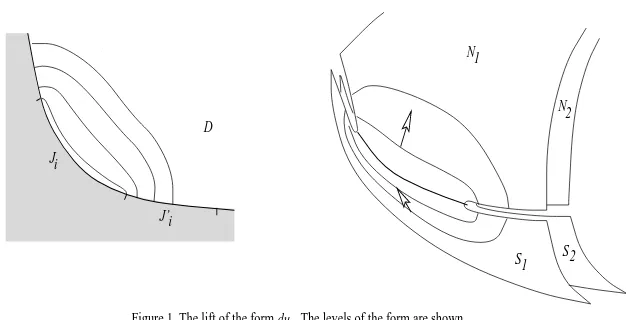
J’i D
Figure 1. The lift of the form du . The levels of the form are shown as solid lines in D ; the dotted lines show the levels of its orthogonal form.
N1
S1 N2
S2
Figure 1: Figure 1. The lift of du. The solid lines denote the levels of u onM; the dotted lines — the levels of the orthogonal form.
Proof:
To start the proof we will construct a linear mapping from the space V of locally constant functions onI=∐iIito the space of harmonic 1-forms onM. Forx= (x0, . . . , xN)∈V, letux
be the continuous function on the upper halfplaneU ⊂C¯ which has the following properties:
• The function is harmonic in the interiority ofU;
• The restriction ofuxtoJi is identicallyxi;
• The normal derivative ofuat the points of∂U ∼=RP1− ∪iJ
i vanishes.
The existence of such a function is standard; one could define ux as the expected value of
thexI, where I is the number of the first of the intervalsJi hitted by the reflected Brownian
motion inU.
Letf : ¯C→U be the folding of the complex sphere to the upper halfplane,x+iy7→x+i|y|.
The composite mapping of the hyperelliptic curve M to U given by k = f ◦p is smooth (and even conformal) outside the preimage of the real projective line RP⊂C¯. On this set
M−k−1(RP) =N1∪S1∪N2∪S2 the mappingk preserves orientation onN’s and reverses
it onS’s. Define the 1-form on this set as
ωx=k∗(dux) onN1∪S2 and ωx=−k∗(dux) onN2∪S1.
Lemma 2.3 The formωx extends to a smooth harmonic form onM (also denoted by ωx).
Proof:
Indeed, the continuity of ωx outside of the ramification points of p (that is, preimages of
ai, bi’s) is clear from the fact that the annulator of dux is tangent to the real line at points of
Ji and orthogonal to it at points ofJi′ (see Figure 1).
Further, the fact thatωxis harmonic at the interior points of the preimages of intervalsJiorJi′
(that is, outside the ramification locus{p−1(a
from the symmetry principle. The fact that the ramification points are removable singularities follows from the boundedness of the integral ofωx, (which is clearly exact in the neighborhood
of each of the ramification points).
Thep-preimage of the segmentJiis a smooth closed curve inM. We fix the orientation of this
curve by demanding that it coincides with the lift of the natural orientation of∂U =RPto N1∪S1. This defines an element ofH1(M,Z). We will denote this element asBi. Analogously,
we will denote asAithe cycle corresponding to the preimage ofJi′oriented in accordance with
the lift from∂U to N1∪S2.
The integration contour splits into two parts, one along the preimage ofJ′
i inN1∪S2, another
by definition, just by a bounded term from the evaluation of ¯p∗(a) on the cycle in H
1(M,Z)
obtained by closing the trajectory of the Brownian motionw∈M run to the timetsuch that τ(t) =T. Letx=s−1(a), withsdefined in 2.6. Then the (closed) 1-formω
xrepresents ¯p∗(a)
under the de Rham isomorphism. Therefore, (Sc(T), a) differs just by a bounded term from I(t) =R
{w(s)}0≤s≤tωx. The processI(t) is a martingale asωxis harmonic, and its characteristic
isRt
0|ωx(w(s))|2ds. Therefore, I(t)/tconverges a.e. to a normal random value with variance 1
SM
R
M|ωx|2vol. Applying Proposition and the fact that Z
(M covers Dfourfold) we obtain the desired result.
2.10. Example. For the rectangular field of size a×b and I1,2 being the b-sides, (and
standard metric) one finds the variance of the asymptotical scoreξisa−2. This is, of course,
of little surprise, as in this case the score Sc(T) is just some rounding ofw(T)/b, wherewthe 1-dimensional Brownian motion.
We notice here that any disk D with just two marked arcs on its boundary can be mapped conformally onto one of the rectangular areas with the intervals being the opposite sides. Moreover, one can adjust the sizes to preserve the area under this mapping.
3
Inverse Problem
3.1 Firstly, the Lemma 2.2 implies that the energy formQis an invariant of the conformal class of the metricgonly. Therefore, it cannot distinguish between ‘soccer fields’ differing by a conformal diffeomorphism and the inverse problem can be meaningfully posed only if one fixes one within each equivalence class. As was mentioned, one can choose the upper half planeU on the Riemannian sphere ¯S=CP1as D provided with its standard (Fubini-Study) metric.
The unspecified data then are the positions of the ‘goalposts’ {ai, bi}i=0,...,N, ai, bi ∈ RP1.
These positions form, apparently, a 2(N+ 1)-dimensional familyC(diffeomorphic toS1 times
a 2N+ 1-dimensional open simplex). The groupP SL(2,R) of conformal diffeomorphisms of
U is three-dimensional, and the associated Teichm¨uller space is a cell of dimension 2N−1,
T =C/P SL(2,R) ∼=R2N−1. The best way to introduce coordinates on T is to employ the
The parameterscij are real, invariant with respect to automorphisms ofU and take values in
R>1. Clearly, they determine an embedding ofT into theRn
>1for some largen.
3.2 The energy form Q is a function onT with values in the space of quadratic formsQ on the (N+ 1)-dimensional real vector spaceV, which have a one-dimensional kernel and are nonnegative definite (we will denote this space as Sym0(V)). The set of such quadratic forms is a cell of dimension N(N−1)/2. The dimension of the image is not less than that of the source and one can ask whether the energy form defines an embedding of the Teichmueller space. If this is the case, one can solve the inverse problem unambiguously.
3.3 Remark. The question about the properites of the energy mappingE :T →Sym0(V) was raised by Colin de Verdi`ere [1] in connection with his studies of the energy forms of plane electric circuits.
3.4 The main result of this section is that the energy functional is indeed an embedding. This follows quite easily from the next Proposition.
LetM be the hyperelliptic curve constructed in the previous section andAi(Bi), i= 0, . . . , N
be the cycles defined in 2.8. The cycles Ai, Bi′ = Pi
j=1Bj, i = 1, . . . , N form a basis in
the integer homologies H1(M,Z) with respect to which the intersection form is standard: hAi, Bj′i=δij;hAi, Aji=hBi′, Bj′i= 0.
iωj is called the period matrix (of the curveM)
and determines the Jacobian variety of the curve M: J(M) =CN/L, L={n+Zm,n,m∈
ıbe the operator defining the complex structure onU. The 1-formdux◦ıis again harmonic.
The annulator of this form is tangent to ∂U at points of intervalsJ′
i and orthogonal to it at
points of ∂U (as follows from the opposite behavior ofdux). The standard calculation shows
whence Z
The properties of the form duxı stated above show that its lift from U to M, with properly
adjusted signs on different branches ofk(we set it to be the lifting on N1∪S1 and opposite
to it onN2∪S2), we obtain, analogously to the case ofωx, a smooth harmonic form onM.
One can check immediately that this form coincide withωxı(where this timeıis the complex
structure on M). Therefore the form ωC
x = ωx−iωxı is a holomorphic 1-form on M. Its
integrals over a cycle Ai are, obviosly, the integrals ofωx over it, as theωxı part vanishes on
the lifts of the vectors tangent to intervalsJ.
It follows that for xi = (1/2)(e0+PNj=i+1ej), ej the standard basis vectors inV, the
cor-By the definition, the entries of the period matrixZ are
zij =
Combining all together we obtain the claimed formula.
As a corollary we immediately obtain the solutiuon of our inverse problem:
Theorem 3.1 The energy map associating the formQto the data(U, g,{I}i)(g=dx2+dy2)
is a proper imbedding of the Teichm¨uller space T into the space Sym0(V). Proof:
The main claim, that the energy map is one-to-one, follows immediately from the Torelli theorem. Indeed, by the Proposition , the formQdefines the period matrix and thence the Jacobian. By Torelli theorem, the curveM can be unambiguously reconstructed formJ(M). In our case, the curve is hyperelliptic, and admits the unique (up to an automorphism in the image) 2-to-1 holomorphic map toCP1. The critical values of the map are just the numbers ai, bi, i= 0, . . . , N, up to an automorphism ofCP1, and, apparently, define the interval system {I}i.
In fact, one can give a pretty detailed description of the image of the Teichmueller space using the theory in [5]. Indeed, givenZ one can form 2N theta constants
θ[η
be used to find the cross ratios parametrizingT: each squared cross ratioc2
ij can be expressed
(via Frobenius formulae) as some ratio of fourth degrees of certain theta-constants [5] p. 3.136. In our situation we are bounded by the requirement that all the cross ratios are real. One sees immediately that it follows from the reality of the theta constants; inversely, the reality of cross-ratios results in the reality ofiZ and therefore in that of the theta constants (as each term in the series defining them is real).
The properness of the energy mapping is also immediate from the Frobenius formula.
4
Concluding Remarks
The results of the previous section yield quite of lot of different corollaries and generalizations. 4.1 Returning to the initial motivation of this study, the soccer field, the Theorem implies, that given the size of the soccer field and assuming that the goalposts are placed symmetrically on the opposite sides of it, the variance of the asymptotic score determines unambigously their width. This is obvious, as the (only) cross ratio involved is that of the images of the goalposts under the conformal mapping taking the field to the upper half plane, and it depends monotonously on the width of the goalposts.
4.2 The results of this paper can be easily extended to the case when the metric has sin-gularities, provided that the total area of the domain remains finite. If the singularities are strong enough, so that the area becomes infinite, we arrive at various generalizations of the results of [3]. The original result of Kozlov, Pitman and Yor describes the case when M has genus 1 and the metricg is the smooth one times a positive function which has at two points (preimages of infinity onM) poles of order 2. Nearly all the time, the trajectory of the motion wanders near these singular points and the characteristic of the integral of any harmonic on M form is, asymptotically, a local time processL0
t at zero for the Bessel process (of order 2).
An immediate generalization can be obtained if one considers an algebraic curveM, a rational functionf :M→Con it and the Riemannian metric onM given by the lift ofdx2+dy2via
f. One can see quite easily that the resulting distribution of the asymptotical score (scaled by
√
logt) has the Laplace transform (1 + (λ, QHλ))−1 for the quadratic formQHdefined in 2.6.
Similarly, one can address the question about the metrics with singularities of other orders. Once again, this can be solved by finding the asymptotical distribution of the local time at zero for the Bessel process of relevant order. Notice, however, that the order of the pole cannot be larger than two: in this case the process is transient, the local time remains finite and one cannot apply the ergodic theorems. Geometrically, this corresponds to Riemannian surfaces with nonempty killing boundary.
References
[1] Y. Colin de Verdi`ere, R´eseaux ´electriques planaires I, Comm. Math. Helv.,69, 351-374 (1994).
[2] Ph. Griffiths, J. Harris,Principles of Algebraic Geometry, Wiley (1979).
[3] S. Kozlov, J. Pitman, M. Yor. Wiener football, Probab. Theory Appl., 40, 530-533 (1993).
[4] T.J. Lyons, H.P. McKean, Winding of the plane brownian motion, Adv. Math., 51, 212-225 (1984).
[5] D. Mumford,Tata lectures on theta. II, Birkh¨auser, Boston, 1984.
[6] J. Pitman, M. Yor Asymptotic laws of planar Brownian motion,Ann. Probab. 14, 733-779 (1986) and17, 965–1011 (1989)