ELECTRONIC COMMUNICATIONS in PROBABILITY
BALANCED RANDOM TOEPLITZ AND HANKEL MATRICES
ANIRBAN BASAK1
Department of Statistics, Stanford University, Stanford, CA 94305, USA email: [email protected]
ARUP BOSE2
Statistics and Mathematics Unit, Indian Statistical Institute, 203 B. T. Road Kolkata 700108, INDIA email: [email protected]
SubmittedJanuary 10, 2010, accepted in final formApril 08, 2010
AMS 2000 Subject classification: Primary 60B20, Secondary 60F05, 62E20, 60G57, 60B10. Keywords: Random matrix, eigenvalues, balanced matrix, moment method, bounded Lipschitz metric, Carleman condition, almost sure convergence, convergence in distribution, uniform inte-grability.
Abstract
Except for the Toeplitz and Hankel matrices, the common patterned matrices for which the limiting spectral distribution (LSD) are known to exist share a common property–the number of times each random variable appears in the matrix is (more or less) the same across the variables. Thus it seems natural to ask what happens to the spectrum of the Toeplitz and Hankel matrices when each entry is scaled by the square root of the number of times that entry appears in the matrix instead of the uniform scaling by n−1/2. We show that the LSD of these balanced matrices exist and derive integral formulae for the moments of the limit distribution. Curiously, it is not clear if these moments define a unique distribution.
1
Introduction and main results
For any (random and symmetric) n×nmatrix B, letµ1(B), . . . ,µn(B)∈R denote its
eigenval-ues including multiplicities. Then theempirical spectral distribution(ESD) ofB is the (random) distribution function onRgiven by
FB(x) =n−1#
n
j:µj(B)∈(−∞,x], 1≤j≤n
o
.
1SUPPORTED BY MELVIN AND JOAN LANE ENDOWED STANFORD GRADUATE FELLOWSHIP FUND
2RESEARCH SUPPORTED BY J.C.BOSE NATIONAL FELLOWSHIP, DEPARTMENT OF SCIENCE AND TECHNOLOGY,
GOVERNMENT OF INDIA
For a sequence of randomn×nmatrices{Bn}n≥1if asn→ ∞, the corresponding ESDs FBn
con-verge weakly (either almost surely or in probability) to a (nonrandom) distributionF in the space of probability measures onR, thenF is called thelimiting spectral distribution(LSD) of{B
n}n≥1. See Bai (1999)[1], Bose and Sen (2007)[6]and Bose, Sen and Gangopadhyay (2009)[5]for de-scription of several interesting patterned matrices whose LSD exist. Examples include the Wigner, the circulants, the Hankel and the Toeplitz matrices. For the Wigner and circulant matrices, the number of times each random variable appears in the matrix is same across most variables. We may call them balancedmatrices. For them, the LSDs exist after the eigenvalues are scaled by n−1/2.
Consider then×nsymmetric Toeplitz and Hankel matrices with an i.i.d. inputsequence {xi}. For these matrices when scaled byn−1/2, the LSDs exist. The limits are symmetric about 0, are non-Gaussian and have unbounded support with LSD for the Hankel matrices being not unimodal. Further the ratio of the (even) moments of the LSD to the standard Gaussian moments tend to 0 as the order increases. See Bryc, Dembo and Jiang (2006)[7]and Hammond and Miller (2005)[8]. Not much more is known about these LSDs. However, these matrices are unbalanced. It seems natural to consider the balanced versions of the Toeplitz and Hankel matrices where each entry is scaled by the square root of the number of times that entry appears in the matrix instead of the uniform scaling byn−1/2. Define the (symmetric) balanced Hankel and Toeplitz matricesBHnand BTnwith input{xi}as follows:
BHn =
x1 p 1 x2 p 2 x3 p 3 . . .
xn−1
p n−1
xn p n x2 p 2 x3 p 3 x4 p 4 . . .
xn
p n
xn+1
p n−1 x3 p 3 x4 p 4 x5 p 5 . . .
xn+1
p n−1
xn+2
p n−2 ..
. xn
pn pxn+1 n−1
xn+2
p
n−2 . . . x2n−2
p 2
x2n−1
p 1 . (1.1)
BTn =
x0 p n x1 p n−1 x2 p
n−2 . . . xpn−2
2 xpn−1
1 x1
p n−1
x0
p n
x1
p
n−1 . . . xpn−3
3 xpn−2
2 x2
p n−2
x1
p n−1
x0
p n . . .
xpn−4
4 xpn−3
3 ..
. xpn−1
1 xpn−2
2 xpn−3
3 . . . x1
p n−1
x0 p n . (1.2)
Strictly speakingBTnis not completely balanced, with the main diagonal being unbalanced com-pared to the rest of the matrix. The main diagonal has all identical elements and making BTn balanced will shift its eigenvalues by x0/
p
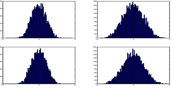
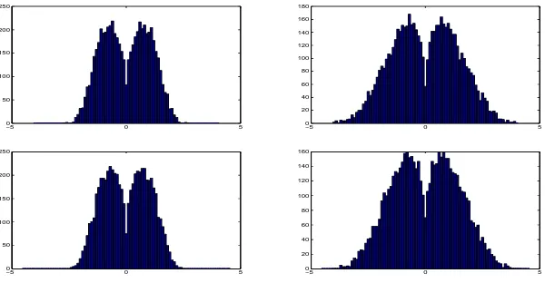
2nwhich in the limit will go to zero and hence this does not affect the asymptotic behavior of the eigenvalues. We use the above version because of the convenience in writing out the calculations later. Figures 1 and 2 exhibit the simulation results for the ESDs of the above matrices. We prove the following theorem. A primitive version of this result appears in Basak[3].
Theorem 1. Suppose{xi}are i.i.d. with mean0and variance1. Then almost surely the LSDs, say BT and BH of the matrices BTnand BHnrespectively, exist and are free of the underlying distribution of the{xi}.
BT and BH have unbounded support, are symmetric about zero and have all moments finite. Both LSDs are non-Gaussian. The integral formulae for the moments are given in (2.10) and (2.12) in Section 2.5 after we develop the requisite notation to write them out. It does not seem to be apparent if these moments define a distribution uniquely. Establishing further properties of the limits is a difficult problem.
The main steps in the proof may be described as follows:
(1) In Section 2.1 we first show that we may restrict attention to bounded{xi}and hence in the later sections, we assume this to be the case.
(2) In Sections 2.2–2.4 we develop the trace formula for moments, some related notions and results to reduce the number of terms in the trace formula. In Section 2.5 we show that the expectedmoments of the ESD of{BTn}converge. However, it does not seem to be straightforward to show that this limiting sequence uniquely determines a distribution. Even if it did, it is not clear how the convergence of the expected moments can be sharpened to convergence of the ESD itself. If we pull out the usual scalingn−1/2, the scaling for the(i,j)th entry is[1−|i−j|
n ]−
1/2whose maximum isn1/2. This unboundedness creates problems in the usual argument.
(3) In Section 2.6 we discuss a known approximation result. (4) Fix any ǫ > 0. LetBTǫ
n denote the top-left⌊n(1−ǫ)⌋ × ⌊n(1−ǫ)⌋ principal sub-matrix of BTn. The Lévy distance betweenFBTn andFBT
ǫ
n is less thanǫ. Since these truncated matrices are
well behaved, we have convergence ofFBTnǫ to a non-random distributionBTǫ almost surely, and
also the corresponding expected moments follow by the same arguments as for the usual Toeplitz matrices. This limit is uniquely determined by its moments. This is done in Section 2.7.
(5) In Section 2.8 we show by using results derived in (3) that asǫ→0, the spectral measures ofBTǫconverge to someFBT and this is the LSD of{BTn}. We finally use a uniform integrability argument to conclude that the moments ofFBT are same as those obtained in (2) above.
A similar proof works for the balanced Hankel matrix by defining the truncated Hankel matrix obtained by deleting the first⌊nǫ/2⌋and last⌈nǫ/2⌉rows and columns fromBHn.
2
Proof of Theorem 1
2.1
Reduction to the uniform bounded case
Lemma 1. Suppose for every bounded, mean zero and variance one i.i.d. input sequence{x0,x1,x2, . . .},
{FBTn}converges to some non-random distribution F a.s. Then the same limit continues to hold even
if the{xi}are not bounded. All the above hold for{FBHn}as well.
We make use of thebounded Lipschitz metric. It is defined on the space of probability measures as:
dB L(µ, ν) =sup
¨Z
f dµ−
Z
f dν:||f||∞+||f||L≤1
«
We also need the following fact. This fact is an estimate of the metric distancedB L in terms of trace. A proof may be found in Bai and Silverstein (2006)[2]or Bai (1999)[1].
Fact 1.SupposeA,Baren×nsymmetric real matrices. Then
dB L2 (FA,FB)≤ 1
n n
X
i=1
|λi(A)−λi(B)|
!2
≤ 1
n n
X
i=1
(λi(A)−λi(B))2≤ 1
nTr(A−B)
2. (2.1)
Proof of Lemma 1. For brevity, we deal with only the balanced Toeplitz case. The same arguments work for the balanced Hankel matrices. For any eventA, defineI(A)as the indicator of the setA so that it is zero or one according as the eventAdoes not or does happen. For t>0 define
µ(t)d e f= E[x0(I|x0| ≤t)], σ2(t)d e f= Var(x0I(|x0| ≤t)) =E[x02I(|x0| ≤t)]−µ(t)2, x∗i = xiI(|xi| ≤t)−µ(t)
σ(t) =
xi−¯xi
σ(t) , where ¯xi=xiI(|xi|>t) +µ(t) =xi−σ(t)x
∗ i.
Let{BTn∗}be the balanced Toeplitz matrix for the input sequence{x∗i}and{ÝBTn}be the same for the input sequence{¯xi}. It is clear that{xi∗}is a bounded, mean zero, variance one i.i.d. sequence. Hence by our assumption,FBTn∗converges to a non-random distribution functionF a.s. Using Fact
1,
d2B L(FBTn,FBTn∗) ≤ 2d2
B L(F
BTn,Fσ(t)BTn∗) +2d2
B L(F BT∗
n,Fσ(t)BTn∗) ≤ 2
nTr[(BTn−σ(t)BT ∗ n)
2] +2
n(1−σ(t))
2Tr[(BT∗ n)
2].
Now using the strong law of large numbers, we get 1
nTr[(BT ∗ n)
2] = 1 n
X
i,j
x
∗ |i−j|
p
n− |i−j|
2
= 1
n n× x∗
0 2
n +2(n−1)× x∗
1 2
(n−1)+· · ·+2×
x∗n−12 1
!
≤ 2
n(x ∗ 0 2
+x1∗2+· · ·+x∗n−12)a.s.→2E(x0∗2) =2. Note that 1−σ(t)→0 ast→ ∞. Similarly,
1
nTr[(BTn−σ(t)BT ∗ n)
2] = 1 nTr[
Ý
BT 2
n]
= 1
n
X
i,j
x¯|i−j|
p
n− |i−j|
2
= 1
n
n× ¯x
2 0
n +2(n−1)× ¯ x21
(n−1)+· · ·+2×
¯ x2
n−1 1
≤ 2
n(¯x 2
0+· · ·+¯x 2 n−1)
a.s.
→2E[x¯20] =1−2µ(t)2−σ2(t)→0 as t→ ∞. Hence combining the above arguments, we get lim supndB L(FBTn,FBTn∗)→0 a.s. as t→ ∞. This
2.2
Moment and trace formula
We need some notation to express the moments of the ESD in a way which is convenient for further analysis.
Circuit and vertex: Acircuitis any functionπ:{0, 1, 2, . . . ,h} → {1, 2, . . . ,n}such that π(0) =
π(h). Anyπ(i)is avertex. A circuit depends onhandnbut we will suppress this dependence. Define two functionsLTandLH, which we calllink functions, by
LT(i,j) =|i−j| and LH(i,j) =i+j−1. (2.2) Also forL=LH orLT, as the case may be, define
Xπ=xL(π(0),π(1))xL(π(1),π(2))· · ·xL(π(h−2),π(h−1))xL(π(h−1),π(h)).
Also define
φT(i,j) =n− |i−j| and φH(i,j) =min(i+j−1, 2n−i−j+1), (2.3) φn
T(x,y) =φ∞T(x,y) =1− |x−y|, (2.4) φn
H(x,y) =min(x+y− 1
n, 2−x−y+ 1 n),φ
∞
H(x,y) =n→∞limφ n
H(x,y). (2.5) Finally, for any matrix B, letβh(B)denote the hth moment of its ESD. Then thetrace formula implies
1
nTr[BTn]
h = 1 n
X
1≤i1,i2,...,ih≤n
Y
1≤j≤h−1 xLT(i
j,ij+1)
p
φT(ij,ij+1)
× xLT(ih,i1)
p
φT(ih,i1) (2.6)
E[βh(BTn)] = E[1
nTr(BTn) h] = 1
n
X
π:πcircuit
EXπ
Q
1≤i≤h
p
φT(π(i−1),π(i)). (2.7)
1
nTr[BHn]
h = 1 n
X
1≤i1,i2,...,ih≤n
Y
1≤j≤h−1 xLH(i
j,ij+1)
p
φH(ij,ij+1)
× xLH(ih,i1)
p
φH(ih,i1)
(2.8)
E[βh(BHn)] = E[ 1
nTr(BHn) h] = 1
n
X
π:πcircuit
EXπ
Q
1≤i≤h
p
φH(π(i−1),π(i)). (2.9)
Matched circuits: Any value L(π(i−1),π(i)) is an L value of π and π has an edge of order e(1≤e≤h)if it has anL-valuerepeated exactlyetimes. Ifπhas at least one edge of order one then E(Xπ) =0. Thus only thoseπwith all e≥2 are relevant. Such circuits will be said to be matched.πispair matchedif all its edges are of order two.
is in alphabetical order. For example, ifh= 6, then the partition{{1, 3, 6},{2, 5},{4}}is asso-ciated with w = a bac ba. For a word w, let w[i] denote the letter in the ith position. The notion of matching and order eedges carries over to words. For instance,a baca bcis matched. a bcad baa is non-matched, has edges of order 1, 2 and 4 and the corresponding partition is
{{1, 4, 7, 8},{2, 6},{3},{5}}.
Independent vertex: Ifw[i]is the first occurrence of a letter thenπ(i)is called anindependent vertex. We make the convention thatπ(0)is also an independent vertex. The other vertices will be calleddependentvertices. If a word hasddistinct letters then there ared+1 independent vertices.
2.3
Reduction in the number of terms
Fix an integerh. Define
Π3+
h ={π:πis matched, of lengthhand has an edge of order greater than equal to 3}. SAn
h = 1 n
X
π:π∈Π3+
h
1 h
Q
i=1
p
φA(π(i−1),π(i))
, A=H or T.
Lemma 2. SAn
h →0as n→ ∞for An= Tnor Hn. Hence, only pair matched circuits are relevant while calculatinglimE[βh(An)].
Proof. We provide the proof only forTn. The proof forHnis similar and the details are omitted. Note that
SAn
h =
X
w 1 n
X
π∈Π(w)TΠ3+
h
1
Qh
i=1
p
n− |π(i−1)−π(i)| =X
w
Sh,w say.
It is enough to prove that for eachw,Sh,w→0. We first restrict attention towwhich have only one edge of order 3 and all other edges of order 2. Note that this forceshto be odd. Leth=2t+1 and
|w|=t. Fix the L-values at sayk1,k2, . . . ,kt wherek1is the L-value corresponding to the order 3 edge and leti0be such thatL(π(i0−1),π(i0)) =k1. We start counting the number of possible π’s from the edge(π(i0−1),π(i0)). Clearly the number of possible choices of that edge is at most 2(n−k1). Having chosen the vertexi0, the number of possible choices of the vertex(i0+1)is at most 2. Carrying on with this argument, we may conclude that the total number ofπ’s having L valuesk1,k2, . . . ,kt is at mostC×(n−k1). Hence for some generic constantC,
Sh,w=1
n
X
0≤ki≤n−1
X
π:πhasLvalues
k1 ,k2 ,...,kt
1
(n−k1)
3 2
t
Q
i=2
(n−ki)
≤ 1
n
X
0≤ki≤n−1
C×(n−k1)
(n−k1)
3 2
t
Q
i=2
(n−ki)
= O(
pn)O((logn)t−1)
n →0 asn→ ∞.
In the last step, we have used the facts that Pnk=11
k =O(logn) and for 0<s <1,
Pn
k=1 1 ks =
O(n1−s). It is easy to see that whenwcontains more than one edge of order 3 or more, the order of the sum will be even smaller. This completes the proof of the first part. The second part is immediate sinceE(Xπ) =1 for every pair matched circuit andE(|Xπ|)<∞uniformly over allπ.
2.4
Slope in balanced Toeplitz matrices
Since the Toeplitz matrices have link function L(i,j) = |i− j|, given an L-value and a vertex there are at most two possible choices of the other vertex. Bryc, Dembo and Jiang (2006)[7]and Hammond and Miller (2005)[8] showed that out of these two possible choices of vertices only one choice counts in the limit. We show now that the same is true for the balanced matrices. Let
Πh,+={πpair matched : there exists at least one pair(i0,j0)withπ(i0−1)−π(i0)+π(j0−1)−π(j0)6=0}, DefineΠh,+(w) = Πh,+∩Π(w)and letπ(i−1)−π(i)be theithslope value.
Lemma 3. Letπ∈Πh+and k1,k2, . . . ,khbe the L-values ofπ. Then there exists j0∈ {1, 2, . . . ,h} such that kj0= Λ(k1,k2, . . . ,kj0−1,kj0+1, . . . ,kh)for some linear functionΛ.
Proof.Note that the sum of all the slope-values ofπis zero. Now the sum of the slope-values from the jthmatched pair is 0 if theLvalues have opposite signs while it is 2k
jor−2kjif theLvalues have the same sign. Hence we have f(k1,k2, . . . ,kh) =0 for some linear function f where the coefficient of kj equals 0 if theL values corresponding tokjhave opposite signs while it is±2 if theLvalues corresponding tokjare of the same sign and the slope-values are positive (negative). Sinceπ∈Πh,+, ∃kj6=0 such that theL-values corresponding to the jthpair have the same sign. Let
{i1,i2, . . . ,il}={j: coefficient ofkj=6 0} and j0=max{j: coefficient ofkj6=0}. Thenkj0can be expressed as a linear combinationkj0= Λ(ki1,ki2, . . . ,kil).
Lemma 4. Sh+
d e f
= 1
n
X
π∈Πh,+
1
Qh
i=1
p
n− |π(i−1)−π(i)| →
0 as n → ∞. Hence, to calculate limE[βh(BTn)] we may restrict attention to pair matched circuits where each edge has oppositely signed L-value.
Proof. As in Lemma 2, writeSh+=
P
wSh+,w whereSh+,wis the sum restricted toπ∈Πh,+(w). It
is enough to show that this tends to zero for eachw. Let the correspondingLvalues to thiswbe k1,k2, . . . ,kh. Hence
Sh+,w= 1 n
X
k1 ,k2 ,...,kh
∈{0,1,2,...,n−1}
#{π∈Πh+(w)such thatLvalues ofπare{k1,k2, . . . ,kh}} h
Y
i=1
(n−ki)
.
For this fixed set of L values, there are at most 22hsets of slope-values. It is enough to prove the result for any one such set. Now we start counting the number of possibleπ’s having those slope-values.
By the previous lemma there exists j0 such that kj0 = Λ(ki1,ki2, . . . ,kil). We start counting the
number of possibleπfrom the edge corresponding to theLvaluekj0, say(π(i∗−1),π(i∗)). Clearly
and the index j0are determined as well. Thus for that fixed set we have
Shset+,w ≤ 1
n
X
0≤ki≤n−1
n−kj0
h
Y
i=1
(n−ki)
=1
n
X
0≤ki≤n−1
i6=j0
1 h
Y
i=1
i6=j0
(n−ki) .
Askj0 = Λ(ki1,ki2, . . . ,kil), in the above sumkj0 should be kept fixed which implies that Sh+,w≤ O((logn)h−1)
n →0 asn→ ∞, proving the first part. The second part now follows immediately.
2.5
Convergence of the moments
E
[
β
h(
BT
n)]
and
E
[
β
h(
BH
n)]
We need to first establish a few results on moments of a truncated uniform random variable. For a given random variableX (to be chosen), define (whenever it is finite)
gT(x) =E[φnT(X,x)−
(1+α)]
and gH(x) =E[φHn(X,x)−
(1+α)]
.
Lemma 5. Let x∈Nn={1/n, 2/n, . . . , 1}, α >0and X be discrete uniform on Nn. Then, for some
constants C1,C2,
max{gT(x),gH(x)} ≤C1x−α+C2(1−x+1/n)−α+1/n.
Proof.Note that
g(x) = 1
n n
X
y=1
1
[1− |x− y n|]
1+α= 1 n
X
y<j 1
(1− j−y n )
1+α+ 1 n
X
y>j 1
(1− y−j n )
1+α+ 1 n, wherex= j/nand 1<j<n. For j=1 ornsimilar arguments will go through. Now,
1 n
X
y<j
1− j−y n
−(1+α)
= 1
n j−1
X
t=1
1− t n
−(1+α)
= nα n−1
X
t=n−j+1 t−(1+α)
≤ nα× C1
(n−j+1)α=C1(1−x+1/n)−α. By similar arguments, 1
n
P
y>j 1
(1−y−nj)
1+α≤C2x− α.
By similar calculations gH(x)≤C1x−α+C2(1−x+1/n)−α+1/nand thus the result follows. Lemma 6. Suppose Ui,n are i.i.d. discrete uniform onNn. Let ai ∈ Z, 1 ≤ i ≤ m be fixed and 0< β <1.Let Yn=
m
P
i=1
aiUi,nand Zn=1−Yn+1/n. Then
sup n
E[|Yn|−βI(|Yn| ≥1/n)] + sup n
Proof.First note that
P(|Y
n| ≤M/n) = E
h
P
−M/n≤ m
X
i=1
aiUi,n≤M/n
Ui,n,j6=i0
i
= E
h
P
−M/n− m
X
i=1
i6=i0
aiUi,n≤ai0Ui0,n≤M/n− m
X
i=1
i6=i0
aiUi,n
i
≤(2M+1)/n.
LetU1,U2, . . . ,Umbemi.i.dU(0, 1)random variables. We note that
U1,n,U2,n, . . . ,Um,n
D
=
⌈nU
1⌉ n ,
⌈nU2⌉ n , . . . ,
⌈nUm⌉ n
. Define
ˆ
Yn=
m
X
i=1
ai⌈nUi⌉ n , Y =
m
X
i=1
aiUi and K=
m
X
i=1
|ai|. Then
ˆ
Yn=D Yn and |Yˆn−Y| ≤K/n.
E[|Yn|−βI(|Yn| ≥1/n)] = E[|Yn|−βI(1/n≤ |Yn| ≤2K/n)] +E[|Yˆn|−βI(|Yˆn|>2K/n)]
≤ nβ4K+1
n +E[(|Y| −K/n) −βI(
|Yˆn|>2K/n)]
≤ o(1) +E[(|Y| −K/n)−βI(|Y|>K/n)]
≤ o(1) +
Z
x>K/n
(x−K/n)−βf
|Y|(x)d x.
Now Z
x>K/n
(x−K/n)−βf|Y|(x)d x=
Z∞
0
x−βf|Y|(x+K/n)d x.
It is easy to see that fYvanishes outside[−K,K]. Using induction one can also prove that fY(x)≤
1 for all x. These two facts yield
Z∞
0
x−βf|Y|(x+K/n)d x≤
Z K+K/n
0
x−β2d x=O(1). Hence
sup n
E[|Yn|−βI(|Yn| ≥1/n)]<∞.
The proof of the finiteness of the other supremum is similar and we omit the details.
Lemma 7. Suppose{xi}are i.i.d. bounded with mean zero and variance 1. Thenlim E[βh(BTn)] andE[βh(BHn)]exist for every h.
Proof. From Lemma 2 it follows that E[β2k+1(BAn)]→0 asn→ ∞whereAn=TnorHn. From Lemma 2 and Lemma 4 (if limit exists) we have
lim
n→∞E[β2k(BTn)] =
X
wpair matched lim n→∞
1 n
X
π∈Π∗(w)
EXπ
Qh
i=1
p
φT(π(i−1),π(i))
= X
wpair matched lim n→∞
1 n
X
π∈Π∗∗(w)
1
Qh
i=1
p
whereΠ∗∗(w) ={π: w[i] =w[j]⇒π(i−1)−π(i) +π(j−1)−π(j) =0}. Denotex
i=π(i)/n. LetS={0} ∪ {min(i,j):w[i] =w[j],i6= j}be the set of all independent vertices of the wordw and let maxSbe the maximum of the elements present inS. Define xS={xi:i∈S}. Eachxican be expressed as a unique linear combinationLT
i(xS). LiTdepends on the wordwbut for notational convenience we suppress its dependence. Note that LT
i(xS) = xi fori ∈Sand also summing k equations we get LT
2k(xS) = x0. If w[i] =w[j]then|LiT−1(xS)−LTi(xS)|=|LTj−1(xS)−LTj(xS)|. Thus using this equality and proceeding as in Bose and Sen[6]and Bryc, Dembo and Jiang[7]
we have,
lim
n→∞E[β2k(BTn)] =
X
wpair matched lim n→∞E
I
(LiT(Un,S)∈Nn,i∈/S∪ {2k})
Q
i∈S\{0} φn
T(Li−1(Un,S),Ui))
,
where for eachi∈S,Un,iis discrete uniform onN
nandUn,S is the random vector onRk+1whose co-ordinates areUn,iandUn,i’s are independent of each other. We claim that
lim
n→∞E[β2k(BTn)] =m T 2k=
X
wpair matched
mT2k,w= X
wpair matched E
I
(LiT(US)∈(0, 1),i∈/S∪ {2k})
Q
i∈S\{0} φ∞
T(Li−1(US),Ui))
,
(2.10) where for each i ∈ S, Ui ∼ U(0, 1) and US is an Rk+1 dimensional random vector whose co-ordinates areUiand they are independent of each other. Note that to prove (2.10) it is enough to show that for each pair matched wordwand for eachkthere existsαk>0 such that
sup n
E
I(
LiT(Un,S)∈Nn,i∈/S∪ {2k})
Q
i∈S\{0} φn
T(Li−1(Un,S),Ui))
1+αk
<∞. (2.11)
We will prove that for each pair matched wordw sup
n E
I(
LiT(Un,S)∈Nn,i∈/S∪ {2k},i<maxS)
Q
i∈S\{0} φn
T(Li−1(Un,S),Un,i))
1+αk
<∞.
We prove the above by induction onk. Fork=1 the expression reduces to E
h
1 1−|Un,0−Un,1|
1+αi . Now
E
h 1
1− |Un,0−Un,1|
1+αi
= E
h
E
n 1
1− |Un,0−Un,1|
1+α
Un,0
oi
= E[gT(Un,0)]≤C1E[Un,0−α] +C2E[(1−Un,0)−α] +1/n by Lemma 5. Hence by Lemma 6 we have sup
n E
h
1 1−|Un,0−Un,1|
1+αi
<∞for all 0< α <1.
Suppose that the result is true fork=1, 2, . . . ,t. We then show that it is true fork=t+1. Fix any pair matched wordw0. Note that the random variable corresponding to the generating vertex of the last letter appears only once and hence we can do the following calculations. Let
Bt+1=
ILT
i(Un,S)∈Nn,i∈/S∪ {2(t+1)},i<maxS
Q
i∈S\{0}
(1− |LT
i−1(Un,S)−Un,i|)
Then
E[Bt+1] = E
h
E[Bt+1
Un,i,i∈S\ {it+1}]
i
= E
ILT
i(Un,S)∈Nn,i∈/S,i<maxS\ {it+1}
Q
i∈S\{0,it+1}
(1− |LT
i−1(Un,S)−Un,i|)
1+α
| {z }
Φn
×gT(Un,it+1−1)I[LT
it+1−1(Un,S)∈
N
n]
| {z }
Ψn
.
Letting|| · ||qdenote theLqnorm, by Lemma 5 and Lemma 6, sup n ||
Ψn||q<∞wheneverαq<1. Let us now consider the wordw∗0obtained fromw0by removing both occurrences of the last used letter. We note that the quantityΦnis the candidate for the expectation expression corresponding to the wordw0∗. Now by the induction hypothesis, there exists anαt >0 such that
sup n
E
ILT
i(Un,S)∈Nn,i∈/S,i<maxS\ {it+1}
Q
i∈S\{0,it+1}
(1− |LT
i1(Un,S)−Un,i|)
1+αt
<∞.
Hence sup n ||
Φn||p<∞ if(1+α)p≤(1+αt). Therefore
αt+1+
1+αt+1 1+αt <
1 p+
1
q =1⇒supn
E[ΦnΨn]≤sup n ||
Φn||p||Ψn||q<∞.
This proves the claim for balanced Toeplitz matrices. For balanced Hankel matrices we again use Lemma 5 and Lemma 6 and proceed in an exactly similar way to get
lim
n→∞E[β2k(BHn)] =m H 2k=
X
wpair matched and symmetric
mH2k,w= X
wpair matched and symmetric
E
I(
LiH(US)∈(0, 1),i∈/S∪ {2k}
Q
i∈S\{0}
φH∞(Li−1(US),Ui))
. (2.12)
It may be noted that the above sum is oversymmetricpari matched words. These are words in which every letter appears once each in an odd position and an even position. Using ideas of Bose and Sen (2008)[6]and Bryc, Dembo and Jiang[7] it can be shown that for any pair matched non-symmetric word w, mH2k,w = 0. So the above summation is taken over only pair matched
symmetric words.
2.6
An approximation result
metrizes weak convergence of probability measures on R. Let µ
i, i = 1, 2 be two probability measures onR. The Lévy distance between them is given by
ρ(µ1,µ2) =inf{ǫ >0 : F1(x−ǫ)−ǫ <F2(x)<F1(x+ǫ) +ǫ, ∀x∈R}, whereFi,i=1, 2, are the distribution functions corresponding to the measuresµi,i=1, 2. Proposition 1. (Bhamidi, Evans and Sen (2009)) Suppose An×n is a real symmetric matrix and Bm×mis a principal sub-matrix of An×n. Then
ρ(FA,FB)≤min
n
m−1, 1
.
Let(Ak)∞k=1be a sequence of nk×nkreal symmetric matrices. For eachǫ >0and each k, let(Bǫk)∞k=1 be an nǫk×nǫk principal sub-matrix of Ak. Suppose that for each ǫ >0, F∞ǫ = lim
k→∞F Bǫ
k exists and
lim sup k→∞
nk/nǫk≤1+ǫ. Then F∞=klim →∞F
Akexists and is given by F
∞=limǫ ↓0F
ǫ ∞.
Consider the principal submatrixBTnǫ of BTnobtained by retaining the first⌊n(1−ǫ)⌋rows and columns of BTn. Then for this matrix, since|i−j| ≤ ⌊n(1−ǫ)⌋, the balancing factor becomes bounded. We shall show that LSD of{FBTnǫ} exists for everyǫand then invoke the above result
to obtain the LSD of{FBTn}. A similar argument holds for{BH
n}, by considering the principal sub-matrix obtained by removing the first⌊nǫ/2⌋and last⌈nǫ/2⌉rows and columns.
2.7
Existence of limit of
{
F
BTnǫ}
and
{
F
BHǫn}
almost surely
Clearly, for any fixedǫ >0, we may write 1
nTr[BT ǫ n]h=
1 n
X
π:πcircuit
Xπ
Q
1≤i≤h
p
n− |π(i−1)−π(i)|×
Y
1≤i≤h
I
h
π(i)≤ ⌊n(1−ǫ)⌋
i
(2.13)
and similarly 1
nTr[BH ǫ n]
h= 1 n
X
π:πcircuit
Xπ
Q
1≤i≤h
φH(π(i−1),π(i))
×Y
1≤i≤h
I
h
⌊nǫ/2⌋ ≤π(i)≤ ⌊n(1−ǫ/2)⌋i. (2.14)
Since for everyǫ >0 the scaling is bounded, the proof of the following lemma is exactly the same as the proof of Lemma 1 and Theorem 6 of Bose and Sen (2008)[6]. Hence we skip the proof. Recall that a symmetric word is a pair-matched word where each letter appears exactly once each in an odd and an even position.
Lemma 8. (i) If h is odd,E[βh(BTnǫ)]→0andE[βh(BHnǫ)]→0. (ii) If h is even (=2k), then
lim
n→∞E[βh(BT ǫ n)] =
X
w
pBTǫ(w) =
X
w
Z1−ǫ
0
· · ·
Z1−ǫ
0
| {z }
k+1
Q
i∈/S∪{2k}
I(0≤LiT(xS)≤1−ǫ)
Q
i∈S\{0}
(1− |LTi−1(xS)−xi|)
where the sum is over pair-matched words w. Similarly,
E[βh(BHǫn)]→X
w
pBHǫ(w) =
X
w
Z1−ǫ2
ǫ
2
· ·
Z1−ǫ2
ǫ
2
| {z }
k+1
Q
i∈/S∪{2k}
I(ǫ
2≤L H
i (xS)≤1−ǫ2)
Q
i∈S\{0} φ∞
H(Li−1H (xS),xi)
d xS=β2kHǫ say
where the sum is over all symmetric pair-matched words w. Further, max{βTǫ 2k,β
Hǫ 2k} ≤
2k! k!2k ×ǫ−
k. Hence there exists unique probability distributions FTǫ and FHǫ withβkHǫ andβkHǫ (respectively) as their moments.
The almost sure convergence of{FBTnǫ}and{FBH
ǫ
n} now follow from the following Lemma. We
omit its proof since it is essentially a repetition of arguments given in the proofs of Propositions 4.3 and 4.9 of Bryc, Dembo and Jiang[7]who established it for the usual Toeplitz matrixTnand the usual Hankel matrixHn.
Lemma 9. Fix any ǫ > 0 and let An = Tn or Hn. If the input sequence is uniformly bounded, independent, with mean zero and variance one then
E
h1
nTr(BA ǫ n)
h−E1 nTr(BA
ǫ n)
hi4=O1 n2
. (2.15)
As a consequence, the ESD of BAǫnconverges to FAǫ
almost surely.
2.8
Connecting limits of
{
BT
nǫ}
(resp.
BH
nǫ) and
{
BT
n}
(resp.
BH
n)
From Lemma 8 and Lemma 9, given anyǫ >0, there exists Bǫ such that P(Bǫ) =1 and onBǫ, FBTnǫ⇒FT
ǫ .
Fix any sequence{ǫm}∞m=1decreasing to 0. DefineB=∩Bǫm. Using Proposition 1, onB,F
BTn⇒FT
for some non-random distribution functionFT whereFT is the weak limit of{FTǫm}∞ m=1.
LetXǫm (resp. X) be a random variable with distributionFTǫm (resp. FT) withkth momentsβTǫm
k (resp. βT
k). From Lemma 8, and (2.10) it is clear that for allk≥1, lim
m→∞β Tǫm
2k+1=0 and mlim→∞βT ǫm
2k =mT2k=
X
wpair matched m2k,wT .
From Lemma 7, m2kT is finite for every k. Hence{(Xǫm)k}∞
m=1 is uniformly integrable for every k and lim
m→∞β Tǫm
k = β T
k. This proves thatm T k = β
T
k and so{m T
k} are the moments of F T. The argument forBHnis exactly same and hence details are omitted. The proof of Theorem 1 is now
complete.
References
[1] Bai, Z. D. (1999). Methodologies in spectral analysis of large dimensional random matrices, a review.Statistica Sinica9, 611–677 (with discussions). MR1711663
[2] Bai, Z. D. and Silverstein, J. (2006).Spectral Analysis of Large Dimensional Random Matrices. Science Press, Beijing.
[3] Basak, Anirban (2009). Large dimensional random matrices. M.Stat. Project Report, May 2009. Indian Statitstical Institute, Kolkata.
[4] Bhamidi, Shankar; Evans, Steven N. and Sen, Arnab (2009). Spectra of large random Trees. Available athttp://front.math.ucdavis.edu/0903.3589.
[5] Bose, Arup; Gangopadhyay, Sreela and Sen, Arnab (2009). Limiting spectral distribution of X X′ matrices. Annales de l’Institut Henri Poincaré. To appear. Currently available at http://imstat.org/aihp/accepted.html.
[6] Bose, Arup and Sen, Arnab (2008). Another look at the moment method for large dimen-sional random matrices.Electronic Journal of Probability, 13, 588–628. MR2399292
[7] Bryc, Włodzimierz; Dembo, Amir and Jiang, Tiefeng (2006). Spectral measure of large ran-dom Hankel, Markov and Toeplitz matrices.Ann. Probab., 34, no. 1, 1–38. Also available at http://arxiv.org/abs/math.PR/0307330MR2206341
[8] Hammond, C. and Miller, S. J. (2005). Distribution of eigenvalues for the ensemble of real symmetric Toeplitz matrices.J. Theoret. Probab.18, no. 3, 537–566. MR2167641
−5 0 5
0 50 100 150 200 250
−5 0 5
0 20 40 60 80 100 120 140 160 180
−5 0 5
0 50 100 150 200 250
−5 0 5
[image:14.612.128.426.506.662.2]0 20 40 60 80 100 120 140 160 180 200
−5 0 5 0
50 100 150 200 250
−5 0 5
0 20 40 60 80 100 120 140 160 180
−5 0 5
0 50 100 150 200 250
−5 0 5
[image:15.612.184.484.364.520.2]0 20 40 60 80 100 120 140 160