Gr¨
obner Bases and Generation of Dif ference Schemes
for Partial Dif ferential Equations
Vladimir P. GERDT †, Yuri A. BLINKOV ‡ and Vladimir V. MOZZHILKIN ‡ † Laboratory of Information Technologies, Joint Institute for Nuclear Research,
141980 Dubna, Russia
E-mail: [email protected]
URL: http://compalg.jinr.ru/CAGroup/Gerdt/
‡ Department of Mathematics and Mechanics, Saratov University, 410071 Saratov, Russia
E-mail: [email protected]
URL: http://www.sgu.ru/faculties/mathematics/chairs/alg/blinkov.php Received December 07, 2005, in final form April 24, 2006; Published online May 12, 2006 Original article is available athttp://www.emis.de/journals/SIGMA/2006/Paper051/
Abstract. In this paper we present an algorithmic approach to the generation of fully con-servative difference schemes for linear partial differential equations. The approach is based on enlargement of the equations in their integral conservation law form by extra integral relations between unknown functions and their derivatives, and on discretization of the ob-tained system. The structure of the discrete system depends on numerical approximation methods for the integrals occurring in the enlarged system. As a result of the discretization, a system of linear polynomial difference equations is derived for the unknown functions and their partial derivatives. A difference scheme is constructed by elimination of all the partial derivatives. The elimination can be achieved by selecting a proper elimination ranking and by computing a Gr¨obner basis of the linear difference ideal generated by the polynomials in the discrete system. For these purposes we use the difference form of Janet-like Gr¨obner bases and their implementation in Maple. As illustration of the described methods and al-gorithms, we construct a number of difference schemes for Burgers and Falkowich–Karman equations and discuss their numerical properties.
Key words: partial differential equations; conservative difference schemes; difference al-gebra; linear difference ideal; Gr¨obner basis; Janet-like basis; computer algebra; Burgers equation; Falkowich–Karman equation
2000 Mathematics Subject Classification: 68W30; 65M06; 13P10; 39A05; 65Q05
1
Introduction
It is well-known that finite differences along with finite elements and finite volumes are most important discretization schemes for numerical solving of partial differential equations (PDEs) (see, for example, [1,2,3,4,5,6,7,8]).
Mathematical operations used in the construction of difference schemes for PDEs are sub-stantially symbolic. Thereby, it is a challenge for computer algebra to provide an algorithmic tool for automatization of the difference schemes constructing as well as for the investigation of properties of the difference schemes. One of the most fundamental requirements for a difference scheme is its stability which can be analyzed with the use of computer algebra methods and software [9].
whenever the original PDEs can be written in the integral conservation law form. One of such tools GRIDOP written in Reduce [10, 11] is based on symbolic operator methods and generates conservative finite-difference schemes on rectangular domains in an arbitrary number of independent variables. However, the generation is not entirely automatic. A user of GRIDOP has to specify function spaces together with associated scalar products and define grid operators as finite-difference schemes. Then the user may provide partial differential equations in terms of the defined grid operators or the adjoints of those operators. Under these conditions the package returns the finite-difference equations for the dependent variables.
Besides, a few other applications of computer algebra are known to construct finite-difference schemes [12,13] which, being also not completely automatic, are applicable to PDEs of a certain form.
In this paper we describe a universal algorithmic approach to the automatic generation of conservative difference schemes for linear PDEs with two independent variables admitting the conservation law form. This approach generalizes and extends the observations of paper [14] where it was noticed that a conservative difference scheme can be derived as a compatibility condition for a system of difference equations. The system is composed of a discrete form of the original PDEs taken in the integral conservation law form and of a number of natural integral relations between functions and their partial derivatives. The finite-difference scheme is obtained by elimination of all the partial derivatives from the system. We also show, by the example of Burgers equation, that one can also apply the difference elimination approach to generate of difference schemes without use of conservation law form.
To perform the difference elimination we apply the Gr¨obner bases method invented 40 years ago by Buchberger [15] for polynomial ideals. This method has become the most universal algorithmic tool in commutative algebra and algebraic geometry and found also numerous fruitful applications for computations in certain noncommutative polynomial rings as well as in rings of linear differential operators and differential polynomials [16]. Nowadays, all modern general-purpose computer algebra systems, for example, Maple [17] and Mathematica [18], have special built-in modules implementing algorithms for computing Gr¨obner bases. However, the fastest implementation of these algorithms for commutative polynomial algebra is done in the special-purpose systems Singular [19] and Magma [20]. As to the difference algebra [21], in spite of known for long time (see [22] and references therein) extensions of Buchberger’s algorithm [23] to difference polynomial rings, there are only a few implementations of the algorithm specialized to shift Ore algebra: in the Ore algebra library package of Maple [24], in the libraryOreModules[25] developed using the latter package and in Singular (Plural) [26]. These packages can be used for computing Gr¨obner bases of linear difference ideals and modules, and, in particular, for those linear systems which are considered below.
In the given paper we present, however, another algorithm for computing difference Gr¨obner bases. This algorithm is superior over our Janet division algorithm whose polynomial version [27] in most cases is computationally more efficient than Buchberger’s algorithm [28]. In addition, unlike the above mentioned implementations of Buchberger’s algorithm for the shift Ore algebra, the algorithm described below and its recent implementation in Maple [29] admit a natural extension to nonlinear difference systems exactly in the same way as differential involutive algorithms [30,31, 32]. The algorithm improves our Janet-like division algorithm [33] adapted to linear difference ideals [34]. The improvement includes, in particular, the difference form of the involutive criteria [27] modified for Janet-like reductions. These criteria allow to avoid some useless reductions, and thereby accelerate the computation.
In Section 4 we present an improved version of the algorithm in paper [34] and briefly discuss some relevant computational aspects. Section 5 illustrates our approach to construction of difference schemes by simplest second-order equations – Laplace’s equation, the wave equation, the heat equation, and by the first-order advection equation. In Section 6 we generate several difference schemes for Burgers equation. But for all that, to avoid problems arising in computing of nonlinear Gr¨obner bases, we denote the square of the dependent variable by an extra function. Besides, we characterize some of the constructed schemes by the modified equation method. In Section 7 we consider the two-dimensional quadratically nonlinear Falkowich–Karman equation describing transonic flow in gas dynamics. Here, we succeeded in computing of the nonlinear Gr¨obner basis by hand, and in that way generated the cubic nonlinear difference scheme which possesses some attractive properties. These properties as well as those of the schemes generated for Burgers equation are illustrated by some numerical experiments in Section 8. We conclude in Section 9.
2
Basic idea
It is well-known [4,5,6, 8] that a rather wide class of scalar PDE and some systems of PDEs can be written in the conservation law form
∂v
∂x + ∂
∂yF(v) = 0, (1)
where v is a m-vector function in the unknown n-vector function u and its partial derivatives ux,uy,uxx, . . .. The vector functionF maps Rm intoRm.
By Green’s theorem (curl theorem in the plane), vector PDE (1) is equivalent to the integral relation
I
Γ
−F(v)dx+vdy= 0, (2)
where Γ is an arbitrary closed contour. Approximation of (2) rather than of (1) on a difference grid (balance or integro-interpolation method) is a natural way to generate conservative finite-difference schemes for PDEs of order two and higher.
Throughout this paper we shall consider orthogonal and uniform grids with the grid mesh stepsh1 and h2
xj+1−xj =h1, yk+1−yk=h2 (3)
and denote the grid values of the vector functionu(x, y) and all its partial derivatives occurring in (2) by
u(x, y) =⇒u(xj, yk)≡ujk, ux(x, y) =⇒ux(xj, yk)≡(ux)jk,
uy(x, y) =⇒uy(xj, yk)≡(uy)jk, uxx(x, y) =⇒uxx(xj, yk)≡(uxx)jk, (4) · · · ·
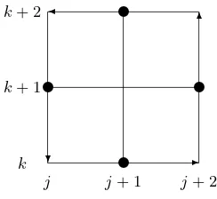
Choose the integration contour as follows (see Fig.1) and add all the related integral relations between the dependent vector variable and its partial derivatives:
Z xj+2
xj
uxdx=u(xj+2, y)−u(xj, y),
Z yk+2
yk
uydy=u(x, yk+2)−u(x, yk),
Z xj+2
xj
uxxdx=ux(xj+2, y)−ux(xj, y),
Z yk+2
yk
uxydy=ux(x, yk+2)−ux(x, yk), (5)
✲ ✻ ✛
❄
✉
✉ ✉
✉ k
k+ 1 k+ 2
j j+ 1 j+ 2
Figure 1. Integration contour on grid.
To obtain a source system of discrete equations for constructing of a difference scheme, we consider numerical approximations of the integral equations (2) for the contour of Fig.1 and of the relations (5) in terms of the grid unknowns (4). Although generally one can use different numerical approximations for the integral equations in (2) and (5), we apply here for all these equations the simplest rectangle (midpoint) rule
F(v)j+1k+2−F(v)j+1k+ (vj+2k+1−vj k+1) = 0,
(ux)j+1k·2h1 =uj+2k−uj k, (uy)j k+1·2h2=uj k+2−uj k, (6) · · · ·
Thereby, we obtained system (6) of difference equations in grid unknowns (4). In doing so, the number of scalar equations added to the (vector) integral equation (2) corresponds to the number of proper partial derivatives of order less than or equal to the order of partial derivatives involved in the integrand of (2).
It follows that eliminating from (6) all the proper grid partial derivatives gives equations con-taining only independent (vector) functionu, and, hence composing a finite-difference scheme. If system (6) is linear, then this difference elimination can always be algorithmically achieved by the Gr¨obner bases method considered in the next section.
It should be noted that generation of finite-difference schemes on grid (3) by the elimination can be also applied to PDEs irrelative to their conservation law properties. Again, one has to add to the initial differential equations, written in terms of grid variables (4), the corresponding number of integral relations (5) and approximate them by numerical quadrature formulas. Such an approach may give more flexibility in generation of distinct difference schemes, and we apply it in Section 4 to the first-order advection equation, and in Section 5 to Burgers equation. Gene-rally, however, for the second-(and higher-) order PDEs admitting the integral conservation law form, the difference scheme obtained directly from the differential form may not be conservative. Besides, the difference elimination based on the integral form is usually more efficient than that based on the differential form. This is because the number of partial derivatives to be eliminated in the former case is smaller than in the latter case. Indeed, the integrand in (2) has the differential order smaller by one than that in (1) whereas computational complexity of the elimination is at least exponential in the number of eliminated variables [35].
3
Dif ference Gr¨
obner bases
A difference ring R is a commutative ring with a unity together with a finite set of mutually commuting injective endomorphisms θ1, . . . , θn of R. Similarly, one defines a difference field.
Elements {y1, . . . , ym}in a difference ring containing Rare said to be difference indeterminates
overR if the set
θk1
1 · · ·θk11yj | {k1, . . . , kn} ∈Zn≥0, 1≤j ≤m
Hereafter we shall consider the ring of functions of n variables x1, . . . , xn with the basis
endomorphisms θi◦f(x1, . . . , xn) =f(x1, . . . , xi+ 1, . . . , xn).acting as shift operators.
The field Q(x1, . . . , xn) of rational functions in {x1, . . . , xn} whose coefficients are rational
numbers is an example of difference field, and we shall assume in the next sections that the coefficients of PDEs belong to this field.
Let K be a difference field, and R := K{y1, . . . , ym} be the difference ring of polynomials over K in variables {θµ◦yk |µ ∈ Zn
≥0, k = 1, . . . , m}. Hereafter, we denote by RL the set of
linear polynomials in Rand use the notations:
Θ :={θµ|µ∈Zn≥0}, degi(θµ◦yk) :=µi, deg(θµ◦yk) :=|µ|:= n
X
i=1 µi,
lcm(µ, ν) :={max{µ1, ν1}, . . . ,max{µn, νn}}, lcm(θµ◦yk, θν ◦yk) :=θlcm(µ,ν)◦yk,
θµ◦yk ⊏ θν◦yk when ν−µ∈Zn
≥0 ∧ |ν−µ|>0. (7)
A difference ideal is an ideal I ⊆R closed under the action of any operator from Θ. If F := {f1, . . . , fk} ⊂R is a finite set, then the smallest difference ideal containing F will be denoted
by Id(F). If for an ideal I there is F ⊂RL such that I = Id(F), then I is a linear difference ideal.
A total ordering≻on the set ofθµ◦yj is arankingif∀i, j, k, µ, ν the following hold:
θiθµ◦yj ≻θµ◦yj, θµ◦yj ≻θν◦yk ⇐⇒ θiθµ◦yj ≻θiθν◦yk.
If |µ| ≻ |ν|=⇒ θµ◦yj ≻θν ◦yk the ranking is orderly. If j > k =⇒ θµ◦yj ≻θν ◦yk the
ranking iselimination.
Given a ranking≻, a linear polynomialf ∈RL\ {0}has theleading termof the forma ϑ◦yj,
ϑ∈Θ, whereϑ◦yj is maximal w.r.t. ≻among allθµ◦yk which appear with nonzero coefficient
in f. lc(f) :=a ∈ K\ {0} is the leading coefficient and lm(f) := ϑ◦yj is the leading (head)
monomial.
A ranking acts inRL as a monomial order. If F ⊆RL\ {0}, then lm(F) will denote the set of the leading monomials and lmj(F) will denote its subset for indeterminateyj. Thus,
lm(F) =∪mj=1lmj(F).
Given a nonzero linear difference idealI = Id(G) and a ranking ≻, the ideal generating set
G={g1, . . . , gs} ⊂RLis a Gr¨obner basis[22,23] ofI if
∀f ∈I∩RL\ {0}, ∃g∈G, θ ∈Θ : lm(f) =θ◦lm(g). (8)
It follows that the head monomial of f ∈I\ {0}, as well as the polynomialf itself, is reducible modulo Gand yields the head reduction:
f −→
g f
′ :=f−lc(f)θ◦(g/lc(g)), f′ ∈I.
Iff′ 6= 0, then its leading monomial is again reducible moduloG, and, by repeating the reduction
finitely many times [16,22,23] we obtainf −→
G 0. Generally, if a polynomialh ∈ RL contains
a term with monomial u and coefficient c 6= 0 such that u = ϑ◦lm(f) for some ϑ ∈ Θ and
f ∈F ⊂RL\ {0}, thenh can be reduced:
h−→
g h
′ :=h−c θ◦(f /lc(f)). (9)
cases ¯h is said to be in the normal form modulo F (denotation: ¯h = N F(h, F)). A Gr¨obner basisG isreducedif
∀g∈G : g=N F(g, G\ {g}).
In our algorithmic construction of reduced Gr¨obner bases we shall use a restricted set of reductions called Janet-like (cf. [33,34]) and defined as follows.
For a finite set F ⊆ RL and a ranking ≻, we partition every lmk(F) into groups labeled
by d0, . . . , di ∈ Z≥0, (0 ≤ i≤ n). Here [0]k := lmk(F) and for i > 0 the group [d0, . . . , di]k is
defined as
[d0, . . . , di]k:={u∈lmk(F)|d0 = 0, dj = degj(u), 1≤j ≤i}.
Now we characterize a monomialu∈lmk(F) by the nonnegative integerλi:
λi(u,lmk(F)) := max{degi(v)|u, v∈[d0, . . . , di−1]k} −degi(u).
If λi(u,lmk(F))>0, thenθsii such that
si:= min{degi(v)−degi(u)|u, v∈[d0, . . . , di−1]k,degi(v)>degi(u)}
is called a difference powerforf ∈F with lm(f) =u.
LetDP(f, F) denotes the set of all difference powers forf ∈F. Now we define the partition of the set Θ into two disjoint subsets
¯
Θ(f, F) :={θµ| ∃θν ∈DP(f, F) : µ−ν ∈Zn≥0}, J(f, F) := Θ\Θ(¯ f, F),
which is similar to the partition of monomials into nonmultiplicative and multiplicative ones in the involutive approach [27].
A finite basisGof I = Id(G) is called Janet-like [33,34] if
∀f ∈I∩RL\ {0}, ∃g∈G, θ∈ J(g, G) : lm(f) =θ◦lm(g). (10)
In full analogy with (9) aJ-reduction is defined as
h−→
g h
′ :=h−c θ◦(f /lc(f)), θ∈ J(f, F), (11)
for polynomial h ∈ RL containing monomial u with coefficient c 6= 0 satisfying u = ϑ◦lm(f) for somef ∈F ⊂RL\ {0}and ϑ∈ J(f, F).
Apparently, any element in the ideal I = Id(G) is J-head reduced to zero by the finite sequence of J-head reductions by elementsg∈Gin the Janet-like basisG:
f −→
g f
′ :=f−lc(f)θ◦(g/lc(g)), θ∈ J(g, G), f′ ∈I. (12)
If the leading monomial ofp∈R\ {0}is notJ-reducible modulo a finite subsetF ⊂R\ {0} we say that p is in the J-head normal form modulo F and writep=HN FJ(p, F). If none of
monomials in p is J-reducible modulo F we say that p is in the (full) normal form modulo F
and write p=N FJ(p, F).
LetGB be a reduced Gr¨obner basis, satisfying [23]:
∀g∈GB : g=N F(g, GB\ {g}). (13)
Let now JB be a Janet basis, and JLB be a Janet-like basis of the same ideal and for the same ranking. Then for their cardinalities the inclusion Card(GB) ≤Card(JLB) ≤Card(JB) holds [27,33]. Here Card abbreviatescardinality, that is, the number of elements.
Whereas the algorithmic characterization of a Gr¨obner basis is zero redundancy of all its
S-polynomials [15,23], the algorithmic characterization of a Janet-like basis Ghas the following form (cf. [33]):
∀g∈G, ϑ∈DP(g, G) : N FJ(ϑ◦g, G) = 0. (14)
These conditions are at the root of the algorithmic construction of Janet-like bases as described in the following section.
4
Algorithm
In this section we present an algorithm for constructing a reduced Gr¨obner basis (8) of the ideal generated by an input set of linear difference polynomials. The algorithm is an improved version of the algorithm in paper [34] and translates to the difference form of the polynomial involutive algorithm [27] modified for the Janet-like reductions.
To apply the difference form of criteria to avoid some unnecessary reductions we need the following definition.
Anancestorof a difference polynomialf ∈F ⊂RL\{0}is a polynomialg∈F of the smallest deg(lm(g)) among those satisfying f =θ◦g modulo Id(F\ {f}) withθ∈Θ. If for all that
deg(lm(g))<deg(lm(f)),
then the ancestorg of f is called proper.
If an intermediate polynomialh that arose in the course of the below algorithm has a proper ancestor g in the intermediate basisG, thenhhas been obtained from g via a sequence of shift operations of the form ϑ◦g where ϑ∈DP(g, G) with lm(ϑ◦g) J-irreducible modulo G. For the ancestor g itself the equality lm(anc(g)) = lm(g) holds.
In the main algorithmGr¨obnerBasisand its subalgorithms we endow every element f ∈G
in the intermediate set of difference polynomialsG(occuring in the setT) with a triple structure of the form:
p={f, g, dpow},
where
pol(p) :=f is the polynomial f itself,
anc(p) :=g is an ancestor of f inG,
dp(p) :=dpow is a (possibly empty) subset of DP(f, G).
The set dpow associated with the polynomialf accumulates all the difference powers for f
Algorithm: Gr¨obnerBasis(F,≺)
Input: F ∈RL\ {0}, a finite set;≺, a ranking
Output: G, a reduced Gr¨obner basis of Id(F)
1: choosef ∈F with the lowest lm(f) w.r.t. ≻ 2: T :={f, f,∅}
3: Q:={ {q, q,∅} |q∈F \ {f} } 4: Q:=HeadReduce(Q, T,≻) 5: while Q6=∅do
6: choosep∈Qwith the lowest lm(pol(p)) w.r.t. ≻ 7: Q:=Q\ {p}
8: if pol(p) = anc(p) then
9: for all{ q∈T |lm(pol(q)) =θµ◦lm(pol(p)), |µ|>0} do
10: Q:=Q∪ {q}; T :=T\ {q}
11: od
12: fi
13: h:=TailNormalForm(p, T,≺) 14: T :=T∪ {h,anc(p),dp(p)}
15: for allq∈T and ϑ∈DP(q, T)\dp(q) do
16: Q:=Q∪ {{ϑ◦pol(q),anc(q),∅}} 17: dp(q) := dp(q)∩DP(q, T)∪ {ϑ} 18: od
19: Q:=HeadReduce(Q, T,≺) 20: od
21: return {pol(f)|f ∈T} or{pol(f)|f ∈T |f = anc(f)}
In the above main algorithmGr¨obnerBasis and its subalgorithms presented below, where no confusion can arise, we simply refer to the triple setT as the second argument inDP,N FJ,
and HN FJ instead of the polynomial set {g = pol(t)|t∈T}. Sometimes we also refer to the
triple pinstead of pol(p). Besides, when we speak of reduction of the triple set Qmodulo triple set T we mean reduction of the polynomial set
{f = pol(q)|q ∈Q}
modulo
{g= pol(t)|t∈T}.
Correctness and termination of algorithm Gr¨obnerBasis can be shown exactly as in the polynomial case [27,33]. Here we only elucidate some related features of the algorithm.
At steps 4 and 19 the J-head reduction is performed for the difference polynomials in Q
modulo those in T. Then the remaining tail reduction is done in line 13 to obtain the (full) J-normal form. Thereby, the main while-loop 5–20 terminates when the conditions (14) hold for the difference polynomial set Gcomposed from the first elements of triples inT
G:={pol(g)|g∈T}, (15)
Furthermore, the main algorithmGr¨obnerBasis together with its subalgorithms presented below ensures that every element in the output Janet-like basis composed from the first elements in the triple setT has one and only one ancestor. This ancestor is apparently irreducible, in the Gr¨obner sense (9), by other elements in the basis. Thereby, those elements in the output basis that have no proper ancestors constitute the reduced Gr¨obner basis (13) that is returned by the main algorithm at the last step 21.
The algorithm HeadReduce invoked in lines 4 and 19 of the main algorithm returns the set Q which, if nonempty, contains part of the intermediate basis J-head reduced modulo T. The reductions are performed by its subalgorithmHeadNormalFormthat is invoked at step 6 of the algorithm.
If algorithm HeadNormalForm returns h 6= 0, then lm(h) does not belong to the initial ideal generated by {lm(pol(f)) |f ∈Q∪T} [27, 36]. In this case the triple {h, h,∅} for h is inserted (line 9) into the output setQ. Otherwise, the output set Qretains the triple p as it is in the input.
In the case when h = 0 and pol(p) has no proper ancestors that is checked at step 14, all the descendant triples for p, if any, are deleted from the intermediate set S at step 16. Such descendants cannot occur in T owing to the choice conditions at steps 1, 6 and to the displacement condition of step 9 in the main algorithm Gr¨obnerBasis. Steps 14–18 serve for the memory saving and can be ignored if the memory restrictions are not very critical for a given problem. In this case all those descendants will be casted away by the criteria checked in the below algorithmHeadNormalForm.
Algorithm HeadNormalForm performs verification (step 3) of J-head reducibility of the input polynomial h modulo the polynomial set (15). This verification consists in searching a difference polynomial (reductor) in the set G defined in (15) such that G yields the reduc-tion (11). If the search fails, that is, there is noJ-reductor, the algorithm returns at step 4 the input polynomial.
For the J-head reducible input polynomial pol(p) that is checked at step 3 of algorithm
HeadNormalForm, the following three criteria are verified at step 9
Criteria(p, g) =C1(p, g)∨C2(p, g)∨C3(p, g), (16)
where
C1(p, g) is true ⇐⇒ lcm(lm(anc(p)),lm(anc(g)))⊏lm(pol(p)),
C2(p, g) is true ⇐⇒ ∃t∈T such that
lcm(lm(pol(t)),lm(anc(p)))⊏lcm(lm(anc(p)),lm(anc(g)))∧
lcm(lm(pol(t)),lm(anc(g)))⊏lcm(lm(anc(p)),lm(anc(g))),
C3(p, g) is true ⇐⇒ ∃t∈T ∧ y∈N ML(t, T) with lm(pol(t))·y= lm(pol(p)),
lcm(lm(anc(p)),lm(anc(t)))⊏lm(pol(p))∧idx(t, T)<idx(f, T),
where idx(t, T) enumerates the position of triplet in setT.
In aggregate, criteria (16) translate (cf. [27,37]) Buchberger’s chain criterion [23] into the linear difference algebra.
In addition, if all difference polynomials in the input setF for the main algorithmGr¨ obner-Basis have constant coefficients, then the set of criteria (16) can be enlarged with one more criterion C4:
C4(p, g) is true for lm(pol(p)) =θ◦yk, lm(pol(g)) =ϑ◦yk ⇐⇒lcm(θ, ϑ) =θ ϑ.
Algorithm: HeadReduce(Q, T,≺)
Input: Qand T, sets of triples;≺, a ranking
Output: J-head reduced setQ moduloT 1: S :=Q
2: Q:=∅
3: while S6=∅do
4: choosep∈S 5: S:=S\ {p}
6: h:=HeadNormalForm(p, T)
7: if h6= 0 then
8: if lm(pol(p))6= lm(h) then
9: Q:=Q∪ {h, h,∅} 10: else
11: Q:=Q∪ {p} 12: fi
13: else
14: if lm(pol(p)) = lm(anc(p))then
15: for all {q∈S|anc(q) = pol(p)}do
16: S:=S\ {q}
17: od
18: fi
19: fi 20: od
21: return Q
Algorithm: HeadNormalForm(p, T,≺)
Input: T, a set of triples;p, a triple; ≺, a ranking
Output: h=HN FJ(p, T), the J-head normal form of pol(p) moduloT 1: h:= pol(p)
2: G:={pol(g)|g∈T}
3: if lm(h) isJ-irreducible moduloGthen
4: return h 5: else
6: take g∈T s.t. lm(h) is J-reducible modulo pol(g)
7: if lm(h)6= lm(anc(p))then
8: if pol(p) =θ◦pol(f) withf ∈T,θ∈DP(f, T) then
9: if Criteria(p, g) then
10: return 0
11: fi
12: fi
13: else
14: while h6= 0 and∃g∈T s.t. lm(h) isJ-reducible by q:= pol(g) do
15: h:=h−lc(h)θ◦(q/lc(q)) with θ∈ J(q, T) and lm(h) =θ◦lm(g)
16: od
17: fi
If all the criteria are false, then theJ-head reduction of h is done by thewhile-loop 14–16 in accordance with the definition of the head reduction in (12).
The last algorithmTailNormalFormcompletesJ-reduction of theJ-head reduced polyno-mial in the input triple by performing itsJ-tail reduction. This algorithm is invoked at step 13 of the main algorithm Gr¨obnerBasis. The tail reduction is performed in the while-loop as a sequence of elementary reductions (11).
Algorithm: TailNormalForm(p, T,≺)
Input: p, a triple such that pol(p) =HN FJ(p, T); T, a set of triples;≺, a ranking
Output: h=N FJ(p, T), the (full) J-normal form of pol(p) modulo T 1: G:={pol(g)|g∈T}
2: h:= pol(p)
3: while h has a term t=aϑ◦yj which isJ-reducible moduloG do
4: take g∈G s.t. ϑ◦yj =θ◦lm(g)
5: h:=h−lc(h)ϑ◦(g/lc(g)
6: od
7: return h
Because of the lack of an appropriate collection of benchmarks for linear finite-difference polynomial systems, the algorithmic efficiency of algorithm Gr¨obnerBasis can be indirectly analyzed by running its polynomial (non-difference) counterpart [27,33] for the extensive bench-marks collection in [38, 39]. Some timings for our polynomial implementation can be found on the Web page [28].
Recently, the algorithm in its difference version was implemented in Maple [29]. Just this implementation was used for generation of linear finite-difference schemes as described in the next sections. Though one needs special and intensive benchmarking for linear difference sys-tems, our first experimenting with the Maple implementation and with that for commutative polynomials gives us a good reason to expect that the following merits revealed for the pure polynomial version [27] hold also for the difference one:
• automatic avoidance of some useless reductions;
• weakened role of the criteria: even without applying any criteria the algorithm is reaso-nably fast;
• smoothed growth of intermediate coefficients;
• fast search of a reductor which provides the elementary Janet-like reduction (11) of a given term. It should be noted that there can be at most one reductor [27];
• natural and effective parallelism.
5
Illustrative examples of PDEs
5.1 Laplace equation
In this section we illustrate the approach of Section 2 to the automatic generation of difference schemes by simplest elliptic, parabolic and hyperbolic equations. To compute Gr¨obner bases providing the elimination of the partial derivatives to construct difference schemes we used the Maple package [29] implementing the algorithms described in the previous section.
We start with the Laplace equation [3,4,5,6,7]
and rewrite it as the conservation law (1)
I
Γ
−uydx+uxdy= 0. (18)
Now we add the relations (5) for the partial derivativesux and uy
Z xj+2
xj
uxdx=u(xj+2, y)−u(xj, y),
Z yk+2
yk
uydy=u(x, yk+2)−u(x, yk). (19)
Thus, we obtain the system of three integral relations (18), (19) for three functions
u(x, y), ux(x, y), uy(x, y).
To discretize this system we choose the rectangular contour of Fig. 1 on the orthogonal and uniform grid (3) with
h1=h2 =h (20)
and use the midpoint integration method for both (18) and (19). This yields the system:
−((uy)j+1k−(uy)j+1k+2) + ((ux)j+2k+1−(uy)j k+1) = 0,
(ux)j+1k·2h=uj+2k−uj k,
(uy)j k+1·2h=uj k+2−uj k.
Rewritten in terms of difference polynomials in the ring Q{u, ux, uy} (see Section 2) it reads:
(θxθ2y−θx)◦uy+ (θ2xθy−θy)◦ux= 0,
2h θx◦ux−(θ2x−1)◦u= 0,
2h θy◦uy−(θ2y−1)◦u= 0.
Computation of the Gr¨obner basis for the elimination ranking (Section 2) withux≻uy ≻uand
θx≻θy gives:
θx◦ux−
1 2h(θ
2
x−1)◦u= 0,
θy◦ux+θx◦uy −
1
2h(θxθy((θ 2
x−1) + (θ2y−1)))◦u= 0,
θ2x◦uy−
1 2h(θ
2
xθy((θx2−1) + (θ2y−1))−θy(θx2−1))◦u= 0,
θy◦uy−
1 2h(θ
2
y−1)◦u= 0,
1 2h(θ
4
xθy2+θ2xθy4−4θ2xθy2+θx2+θy2)◦u= 0.
The latter equation with eliminated ux and uy is the standard difference scheme with the
central approximation of the second-order derivatives in (17) written in double nodes
uj+2k−2uj k+uj−2k
4h2 +
uj k+2−2uj k+uj k−2
4h2 = 0.
Similarly, the trapezoidal integration rule for relations (19) generates the same difference scheme but written in ordinary nodes
uj+1k−2uj k+uj−1k
h2 +
uj k+1−2uj k+uj k−1
❄
✉ ✉
✉ ✉
✻
n n+ 1
j j+ 2
✉ ✉
✲ ✲ ✛ ✛
j+ 1
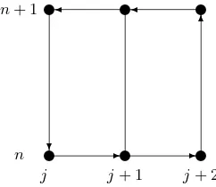
Figure 2. Integration contour for heat equation.
5.2 Heat equation
Consider now the heat equation [3,4,5,6,7,8]
ut+αuxx= 0
in its conservation law form
I
Γ
−αuxdt+udx= 0. (21)
The integrand in (21) contains the only partial derivative ux. Hence we add the single integral
relation
Z xj+1
xj
uxdx=u(xj+1, t)−u(xj, t). (22)
Again we discretizeu(x, t) and ux(x, t) on the orthogonal and uniform grid with the spatial
mesh step h and the temporal mesh step τ, and choose the contour shown in Fig. 2. Then, applying the midpoint rule for the contour integral and the trapezoidal rule for the relation integral we find two difference equations for two indeterminates u, ux in the form
ατ
2(1 +θt−θ
2
x−θtθ2x)◦ux−2h(θxθt−θx)◦u= 0,
h
2(θx+ 1)◦ux−(θx−1)◦u= 0.
By elimination of ux by means of the Gr¨obner basis with ux ≻ u we obtain the famous
Crank–Nicholson scheme [3,4,5,6,7,8,9]
unj+1−un j
τ +α
(unj+1+1−2ujn+1+unj−1+1) + (un
j+1−2unj +unj−1)
2h2 = 0.
The same scheme is obtained for the midpoint integration method applied to (22).
5.3 Wave equation
The wave equation [3,4,5,6,7,8]
utt−uxx= 0
in the conservation law form is given by
I
Γ
Choosing the same grid with the mesh steps (20), the contour of Fig.1and integral relations (19) as are used in Section 5.2 for the Laplace equation (18) and applying the midpoint rule for the contour integral and the trapezoidal rule for the integral relations we obtain the operator equations
(θx−θxθt2)◦ut+ (θx2θt−θt)◦ux= 0,
h
2(θx+ 1)◦ux−(θx−1)◦u= 0,
h
2(θt+ 1)◦ut−(θt−1)◦u= 0.
The Gr¨obner basis method yields the standard difference scheme
unj+1+unj−1−unj+1−unj−1= 0.
5.4 Advection equation
Consider now a simple form of the Advection (or convection or one-way wave) equation [3,4,5,
6,7,8,9]
ut+ν ux = 0, ν = const. (23)
Being of first order, the equation (23) has already the conservation law form (1). By this reason, to generate a difference scheme we shall not convert the equation into the integral form (2). In the latter case one has nothing to eliminate. Instead, we consider equation (23) together with the integral relations:
ut+ν ux = 0,
Z t2
t1
utdt=u(t2, x)−u(t1, x),
Z x2
x1
uxdx=u(t, x2)−u(t, x1). (24)
Discretization ofu,ut and ux on the orthogonal and uniform grid with the mesh steps h and τ
and the explicit integration formula for the upper integral relation in (24) together with the midpoint integration rule for the lower relation give the difference system:
ut+ν ux = 0, τ ut= (θt−1)◦u, 2h θx◦ux = (θx2−1)◦u. (25)
Let us apply the operator θx to both sides of the middle equation in (25) and then use the
Lax method, that is, replaceθx with (θx2+ 1)/2 in the second term of the right-hand side. This
replacement yields
ut+ν ux = 0,
θx◦ut·τ−
θtθx−
θ2
x+ 1
2
◦u= 0,
2θx◦ux·h−(θ2x−1)◦u= 0.
The lexicographical Gr¨obner basis for the elimination rankingut≻ux ≻u withθt≻θx, is
ut+ν ux = 0,
2h θx◦ux−(θ2x−1)◦u= 0,
(2h θxθt−h(θ2x+ 1) +τ(θx2−1)·ν)◦u= 0.
Its last element gives the scheme:
unj+1+1 = u
n
j+2+unj
2 −
ντ(un
j+2−unj)
6
Burgers equation
6.1 Conservation law form
Consider Burgers equation [4,5,8,9] in the form
ut+fx=ν uxx, ν= const, (26)
where we replacedu2 by the flux functionf in order to avoid computation of nonlinear difference
Gr¨obner bases. ν is called the viscosity. This equation exhibits some difficult features from the point of view of simple finite difference schemes due to the term f =u2. Let us, first, convert equation (26) into the conservation law form
I
Γ
(νux−f)dt+udx= 0.
Then choose the contour of Fig. 1and add the integral relation
Z xj+2
xj
uxdx=u(xj+2, t)−u(xj, t).
Denoting as above the temporal and spatial mesh steps byτ andh, and applying the midpoint integration rule we obtain the system:
h(θxθ2t −θx)◦u−τ(θ2xθt−θt)◦(νux−f) = 0,
2h θx◦ux−(θ2x−1)◦u= 0.
Its Gr¨obner basis form for the elimination order withux ≻u≻f and θt≻θx is given by
2ντ h θt◦ux+ 2h2θx(θt2−1)◦u+ 2τ hθt(θx2−1)◦f −ντ θtθx(θ2x−1)◦u= 0,
2h θx◦ux−(θ2x−1)◦u= 0,
2h2θx2(θt2−1)◦u−ντ θt(θx4−2θ2x+ 1)◦u+ 2τ h θtθx(θ2x−1)◦f = 0.
The obtained difference scheme
unj+2+2−un j+2
τ −ν
ujn+4+1−2ujn+2+1+unj+1
2h2 +
fjn+3+1−fjn+1+1
h = 0. (27)
is the standard explicit scheme with forward time and forward space differencing. It is well-known that schemes of this type are unstable [5,8,9]. Furthermore, by using implicit schemes one can provide the von Neumann stability1. However, all such schemes are usually not very
satisfactory when one considers non-smooth or discontinuous solutions (shock waves) of Burgers equation.
6.2 Lax method
To exploit more flexibility and freedom in our difference elimination approach to generation of finite-difference schemes, we go back to the original differential equation (26) and consider it together with the integral relations providing the elimination. For discretization of the relations we combine the midpoint rule for integration over x with the explicit integration over t and apply the Lax method to the last integration:
ut+fx=νuxx, (ut)nj + (fx)nj =ν(uxx)nj,
1
Z
One can also use the trapezoidal rule for the spatial integrations. This derives other schemes. Since there are three spatial integrals in (28), by selecting either the midpoint or the trape-zoidal rule for these integrals, we obtain eight possible variants of the difference schemes. Our computation with the Gr¨obner bases reveals seven different schemes. Apart from (29) there are
2(unj+2+1+ujn+1+1)−(un
Just the scheme (34) is obtained twice in the course of generating eight schemes.
6.3 Two-step Lax–Wendrof f method
Our Gr¨obner basis based technique can also be applied to generate other types of difference schemes. For example, one can generate two-step Lax–Wendroff schemes [41]. Let u and f
denote the values ofuandf on the intermediate time levels. Then, applying again the midpoint rule for the spatial integrals, gives the following difference system:
utnj τ =unj+1−
the Gr¨obner basis contains the Lax–Wendroff scheme
unj+2+1−(un
With all possible combinations of the trapezoidal and midpoint rules one obtains 49 different Lax–Wendroff schemes.
6.4 Dif ferential approximation
To analyze properties of a difference scheme it can be useful to compute its differential ap-proximation [40] that is often called the modified equation(s) of the difference scheme. There are whole classes of different schemes for which their stability properties can be obtained with the aid of the differential approximation [2]. For all that, in many cases, the computation can be easily done with modern computer algebra software. In our research we use Maple [17]. Consider, for example, the schemes (29)–(35).
Their differential approximation for f =u2 and with collection of the coefficients at τ, h2,
h2/τ is given by:
The schemes (29)–(35) differ in the coefficient (∗) ath2only. These coefficients are as follows
(36) 1
Thereby, comparison of differential approximations for schemes (29)–(35) shows that
• all the schemes provide the same order of approximation in τ,h;
• they have identical linear numerical dissipation (viscosity) [4,9] determined byuxxh2/(2τ);
• the schemes possess similar dispersion properties with distinction in the rational coefficients of the differential polynomial inu multiplied byh2.
As to scheme (27), the right-hand side of its differential approximation reads
This explicitly shows instability of the scheme which does not yield linear numerical viscosity. We obtained also analogous results on stability and on close properties for the different Lax–Wendroff schemes of type (36) and its variations due to the choice of different numerical integration rules for the spatial integrals.
6.5 Godunov method
It is especially difficult to simulate numerically nonsmooth and discontinuous solutions which are among most interesting problems in computational fluid and gas dynamics [1, 4, 5, 8]. Most of the known difference schemes fail to handle these singularities. The most appropriate numerical approach to such problems was developed by Godunov [1,42] and based on solving a local Riemann problem [4, 6] as a cornerstone of the Godunov’s scheme generation. There are special numerical Riemann solvers, for example [43], designed for these purposes and for application to computational fluid dynamics.
Instead of the use of numerical Riemann solvers, we apply the Gr¨obner bases technique to generate the Godunov-type scheme for inviscid Burgers equation when ν = 0 in (26). For this purpose we discretize the corresponding system in (28) in the following way
utnj +fxnj = 0,
utnj τ =unj+1−unj,
(fxnj h−(fjn+1−fjn))(fxjn+1h−(fjn+1−fjn)) = 0,
2uxnj+1h=unj+2−unj,
2uxxnj+1h=uxnj+2−uxnj. (37)
Here, the third equation contains in its left-hand side the product of two different solutions for the flux function f of the local Riemann problem [43]. Therefore, we add to the system composed of the original differential equation and discrete forms of the integral relations for partial derivativesut,ux,uxx the nonlinear difference equation onf andfx containing solutions
of the local Riemann problem.
that condition. To do the elimination from the nonlinear system (37) we apply the Gr¨obner factoring approach [44]: if a Gr¨obner basis contains a polynomial which factors, then the com-putation is split into the comcom-putation of two or more Gr¨obner bases corresponding to the factors. In doing so, we choose the elimination ranking
uxx≻ux≻ut≻fx≻f ≻u
and compute two Gr¨obner bases, for every factor in (37). Then we compose the product of two obtained difference polynomials in uand f that gives us the Godunov-type difference scheme:
unj+2+1−un
Consider now the nonlinear two-dimensional Falkowich–Karman equation [45]
ϕxx(K−(γ+ 1)ϕx) +ϕyy = 0 (39)
describing transonic flow in gas dynamics in its non-stationary form
ϕxx(K−(γ+ 1)ϕx) +ϕyy−2ϕxt−ϕtt= 0. (40)
This form can be used to find a stationary solution by the steady-state method. We rewrite equation (40) into the conservation law form
Z tn+1
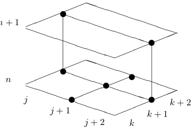
Here we use a grid decomposition of the three-dimensional domain in (x, y, t) into elementary volumes. Fig. 3shows an elementary volume.
Again we add the integral relations for partial derivatives with the use of the trapezoidal integration rule forϕx,ϕy and the midpoint rule forϕt.
Then we obtain the nonlinear operator equations:
Because of nonlinearity in the initial differential equation (40), the difference system obtained is also nonlinear. By this reason the Maple package [29] implementing algorithmGr¨obnerBasis
j+ 2
Figure 3. Cell for Falkowich–Karman equation.
the above described algorithm and with an assistance of Maple to check some intermediate results.
In these calculations we used the lexicographical ranking such that ϕx ≻ϕy ≻ϕt ≻ϕ and
θx≻θy ≻θt. The resulting Gr¨obner basis has the form:
The last element is the finite-difference scheme for equation (40):
(ϕnj+1k−2ϕnj k+ϕnj−1k)·h(ϕnj k−2ϕnj−1k+ϕnj−2k)K−(γ+ 1)
✉
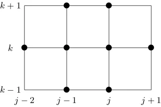
Figure 4. Stencil for stationary Falkowich–Karman equation.
In its stationary form scheme (42)
Dxx(ϕnj k)·
is related to equation (39). Here symbols Dx and Dy are the forward differencing operators
and Dxx and Dyy are the central second-order differencing operators with respect to x and y.
The stencil for scheme (43) is shown in Fig.4.
It should be noted that, unlike the original differential equation (40) which is quadratically nonlinear, both schemes (42) and (43) have the the cubic nonlinearity in the grid function. This is the rigorous algebraic consequence of the difference system (41). In accordance to the well-known fact [46], that algebraic elimination of variables from a nonlinear system leads generally to increase of its degree of nonlinearity.
As an application of this scheme, in the next section we consider an example of one-dimen-sional transonic flow with shock-wave taken from [47].
8
Numerical experiments
8.1 Burgers equation
We used schemes (29), (36) and (38) for numerical simulation in 0 < x < 1 of the following Riemann problem for the inviscid Burgers equation (26) withν = 0
ut+uxu= 0, (44)
and discontinuous initial conditionu(x,0):
u(x,0) =
(
ul, 0< x < 12,
ur, 12 < x <1.
(45)
In (45) the initial data att= 0 is a piecewise-constant function with the state ul on the left of
the discontinuity x = 0 and the state ur on the right of the discontinuity. We consider ν = 0,
since in this case the problem (44), (45) admits the exact solution:
0
Figure 5. Lax scheme (29) with Courant num-ber 0.9.
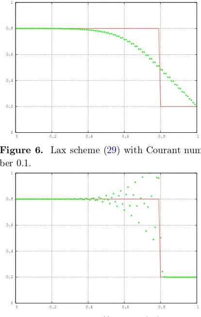
Figure 6. Lax scheme (29) with Courant num-ber 0.1.
Figure 7. Lax–Wendroff scheme (36) with Cou-rant number 0.9.
Figure 8. Lax–Wendroff scheme (36) with Cou-rant number 0.1.
Here H(y) is the Heaviside step function [48] whose derivative is the Dirac delta function:
H(y) =
Physically, the solution (46) defined by the initial condition (45) represents a shock wave which moves with constant speed (ul+ur)/2 without changing its shape.
In our numerical simulation the values oful and ul were chosen as 0.8 and 0.2. The pictures
below demonstrate the numerical solution of the Riemann problem (44), (45) at timet= 2/3. Solid line shows the exact solution (46), and the numerical results are depicted by green dots. For the ratioτ /hof mesh steps which is called Courant (or Courant–Friedrichs–Levy) number [1] we have chosen the two values 0.9 and 0.1.
All schemes are numerically stable. For schemes (29) and (36) their stability is analytically showed by the differential approximation (Section 6.4). Because of the nonlinearity infx in the
third equation of Godunov scheme (38) we did not compute the differential approximation for this scheme.
0 0.2 0.4 0.6 0.8 1
0 0.2 0.4 0.6 0.8 1
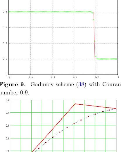
Figure 9. Godunov scheme (38) with Courant number 0.9.
0 0.2 0.4 0.6 0.8 1
0 0.2 0.4 0.6 0.8 1
Figure 10. Godunov scheme (38) with Courant number 0.1.
Figure 11. Initial numerical approximation for equation (39).
Figure 12. Numerical solution of equation (39).
8.2 Falkowich–Karman equation
Now we consider the application of difference scheme (43) to the one-dimensional stationary transonic flow in a channel with a straight density jump [47]. The exact shock-wave solution of equation (39) at 0 ≤x ≤1 is shown in Figs. 11 and 12 by solid red line. Circles depict the numerical data obtained from difference scheme (43). As an initial approximation, the parabola was chosen satisfying the following boundary conditions: at the left, both the function and its derivative are fixed by the values from the exact solution; at the right, the only function is bound to the exact solution.
As one can see from Fig.12, scheme (43) possesses a stable and uniform convergence to the exact shock-wave solution. Because, by its construction, the scheme is fully conservative, it does not reveal non-uniqueness of solutions that is typical for the traditional difference schemes [47]. Moreover, the size of the shock transition zone is just one spatial mesh step that is a conse-quence of preserving at the discrete level of all algebraic properties of the initial PDE (40). This is a result of algebraic difference elimination provided by the Gr¨obner bases method. Another merit of scheme (43) is that it does not involve switches that is typical for computing transonic flow as we already pointed out in Section 7.
This example shows a principal possibility of constructing difference schemes for transonic flow without switches and with the same stencil for both subsonic and supersonic flow.
9
Conclusion
schemes for linear PDEs with two independent variables and with rational function coefficients. Owing to the Gr¨obner bases, this construction is an algorithmic procedure. It consists in elimi-nation of partial derivatives from the system of difference equations composed from a discrete version of the original PDEs (on an orthogonal uniform grid) and numerically approximated integral relations between the unknown functions and their partial derivatives. As this takes place, the difference scheme obtained may depend on the choice of the integration contour and numerical approximations for integral relations.
The method is especially efficient when a PDE or a system of PDEs admits the conservation law form. In this case the difference schemes obtained are fully conservative. The structure of a scheme generated may depend on the choice of integration contour and numerical integration rules. In so doing, it is not clear a priori which integration rule leads to a better scheme.
We also described an efficient algorithm for the construction of Gr¨obner bases for linear difference ideals. The algorithm is based on the concept of Janet-like reductions. Its first implementation in Maple is already available, and we used this implementation in the generation of all linear difference schemes presented in the paper.
For classical linear PDEs such as the Laplace equation, the Heat equation, the Wave equation and the Advection equation our algorithmic technique leads to the well-known finite difference schemes. For Burgers equation we generated several schemes based on the Lax and Lax– Wendroff methods and computed their numerical dissipation and dispersion by the differential approximation (modified equation) method. By example of Burgers equation we also demon-strate that it is possible to combine the Godunov method with Gr¨obner bases to derive a shock capturing scheme.
The non-traditional cubic nonlinear difference scheme generated by our difference elimination method for the Falkowich–Karman equation describing transonic flow in gas dynamics possesses a number of attractive properties in comparison with traditional schemes. Among them there are a stable convergence in time to the exact solution with a one-dimensional shock wave and absence of switches. It should be noted, however, that due to its cubic nonlinearity, scheme (43) has a slower convergence in comparison with the traditional schemes specially optimized for numerical simulation of transonic flows in gas dynamics. By this reason one needs additional research for optimizing nonlinear schemes obtained by the difference elimination.
As we already mentioned in the introduction, algorithm Gr¨obnerBasis admits a generali-zation to polynomial-nonlinear systems of difference equations exactly in the same way as the differential involutive algorithm of paper [32]. In doing so, if every equation in the initial system is linear with respect to the highest ranking difference term and this property of the system is not violated during its completion to involution, then algorithm Gr¨obnerBasis will work correctly and provide the desirable output. Such is indeed the case for system (41). In the most general case of a difference system with polynomial nonlinearity, it can be split into a finite number of subsystems such that every subsystem can be converted into the Gr¨obner basis form by applying our algorithm. The underlying splitting algorithm is a difference analogue of that described in [31]. The latter algorithm is similar to the splitting algorithm implemented in the library packagediffalg in Maple.
The above described approach can be also generalized to PDEs with three and more indepen-dent variables. Thus, if PDEs admit the conservation law form, then one can use multidimen-sional analogues of equations (1) and (2) together with their elementary volume discretization.
Acknowledgements
supported by grants 04-01-00784 and 05-02-17645 from the Russian Foundation for Basic Re-search and by grant 2339.2003.2 from the Ministry of Education and Science of the Russian Federation.
[1] Godunov S.K., Ryaben’kii V.S., Difference schemes. An introduction to the underlying theory, New York, Elsevier, 1987.
[2] Strikwerda J.C., Finite difference schemes and partial differential equations, 2nd ed., Philadelphia, SIAM, 2004.
[3] Ganzha V.G., Vorozhtsov E.V., Numerical solutions for partial differential equations: problem solving using Mathematica, Boca Raton, CRC Press, 1996.
[4] Quarteroni A.,Valli A., Numerical approximation of partial differential equations, 2nd ed., Berlin, Springer-Verlag, 1997.
[5] Thomas J.W., Numerical partial differential equations: finite difference methods, 2nd ed., New York, Springer-Verlag, 1998.
[6] Thomas J.W., Numerical partial differential equations: conservation laws and elliptic equations, New York, Springer-Verlag, 1999.
[7] Samarskii A.A., The theory of difference schemes, New York, Marcel Dekker, 2001.
[8] Morton K.W., Mayers D.F., Numerical solution of partial differential equations, 2nd ed., Cambridge, Cam-bridge University Press, 2005.
[9] Ganzha V.G., Vorozhtsov E.V., Computer-aided analysis of difference schemes for partial differential equa-tions, New York, Wiley-Interscience, 1996.
[10] Liska R., Shashkov M.Yu., Algorithms for difference schemes construction on non-orthogonal logically rect-angular meshes, in Proceedings of ISSAC’91, New York, ACM Press, Addison Wesley, 1991, 419–426.
[11] Liska R., Shashkov M.Y., Solovjov A.V., Support-operators method for PDE discretization: symbolic algo-rithms and realization,Mathematics and Computers in Simulation, 1994, V.35, 173–183.
[12] Fourni´e M., Symbolic derivation of different class of high-order schemes for partial differential equations, in Computer Algebra in Scientific Computing / CASC’99, Springer-Verlag, 1999, 93–100.
[13] K¨oller R., Mohl K.D., Schramm H., Zeitz M., Kienle A., Mangold M., Stein E., Gilles E., Method of lines within the simulation environment DIVA for chemical processes, in Adaptive Method of Lines, Chapmann and Hall, 2001, 371–406.
[14] Mozzhilkin V.V., Blinkov Yu.A., Methods of constructing difference schemes in gas dynamics,Transactions of Saratov University, 2001, V.1, N 2, 145–156 (in Russian).
[15] Buchberger B., An algorithm for finding a basis for the residue class ring of a zero-dimensional polynomial ideal, PhD Thesis, University of Innsbruck, Institute for Mathematics, 1965 (in German).
[16] Buchberger B.,Winkler F. (Editors), Gr¨obner bases and applications, Cambridge University Press, 1998.
[17] http://www.maplesoft.com/
[18] http://www.wolfram.com/
[19] Greuel G.-M., Pfister G., Sch¨onemann H., Singular 3.0. A computer algebra system for polynomial computa-tions, Centre for Computer Algebra, University of Kaiserslautern, 2005,http://www.singular.uni-kl.de/
[20] http://magma.maths.usyd.edu.au/magma/
[21] Cohn R.M., Difference algebra,Tracts in Mathematics, Vol. 17, Interscience Publishers, 1965.
[22] Kondratieva M.V., Levin A.B., Mikhalev A.V., Pankratiev E.V., Differential and difference dimension polynomials. Mathematics and its applications, Dordrecht, Kluwer, 1999.
[23] Buchberger B., Gr¨obner bases: an algorithmic method in polynomial ideal theory, in Recent Trends in Multidimensional System Theory, Dordrecht, Reidel, 1985, 184–232.
[24] Chyzak F., Salvy B., Non-commutative elimination in Ore algebras proves multivariate identities,J. Symbolic Computation, 1998, V.26, 187–227.
[25] Chyzak F., Quadrat A., Robertz D., OreModules: a symbolic package for the study of multidimensional linear systems, in Applications of Time-Delay Systems, Editors J. Chiasson and J.-J. Loiseau, Springer, to appear (seehttp://wwwb.math.rwth-aachen.de/OreModules).
[27] Gerdt V.P., Involutive algorithms for computing Gr¨obner bases, in Computational Commutative and Non-Commutative Algebraic Geometry, Amsterdam, IOS Press, 2005, 199–225, math.AC/0501111.
[28] http://invo.jinr.ru
[29] Gerdt V.P., Robertz D., A Maple package for computing Gr¨obner bases for linear recurrence relations, cs.SC/0509070.
[30] Janet M., Le¸cons sur les Syst`emes d’Equations aux D´eriv´ees Partielles, Cahiers Scientifiques, IV, Paris, Gauthier-Villars, 1929.
[31] Thomas J., Differential systems, New York, American Mathematical Society, 1937.
[32] Gerdt V.P., Completion of linear differential systems to involution, in Computer Algebra in Scientific Computing CASC’99, Editors V.G. Ganzha, E.W. Mayr and E.V. Vorozhtsov, Berlin, Springer, 1999, 115– 137, math.AP/9909114.
[33] Gerdt V.P., Blinkov Yu.A., Janet-like monomial division. Janet-like Gr¨obner bases, in Computer Algebra in Scientific Computing / CASC 2005, LNCS, Springer, 2005, 174–195.
[34] Gerdt V.P., On computation of Gr¨obner bases for linear difference systems, math-ph/0509050.
[35] von zur Gathen J., Gerhard J., Modern computer algebra, 2nd ed., Cambridge University Press, 2003.
[36] Gerdt V.P., Blinkov Yu.A., Involutive bases of polynomial ideals. Minimal involutive bases, Mathematics and Computers in Simulation, 1998, V.45, 519–560, math.AC/9912027, math.AC/9912029.
[37] Apel J., Hemmecke R., Detecting unnecessary reductions in an involutive basis computation, RISC Linz Report Series 02-22, 2002.
[38] http://www-sop.inria.fr/saga/POL
[39] http://www.math.uic.edu/∼jan/demo.html
[40] Shokin Yu.I., Yanenko N.N., Method of differential approximation. Application to gas dynamics, Nauka, Siberian Division, 1985 (in Russian).
[41] Richtmyer R.D., Morton K.W., Difference methods for initial-value problems, 2nd ed., New York, John Wiley & Sons, 1967 (reprinted Krieger Publishing Company, New York, 1994).
[42] Godunov S.K., A finite difference method for numerical computation and discontinuous solutions of the equations of fluid dynamics,Math. Sb., 1959, V.47, 271–306 (in Russian).
[43] Toro E.F., Riemann solvers and numerical methods for fluid dynamics, 2nd ed., Berlin, Springer-Verlag, 1997.
[44] Czapor S.R., Solving algebraic equations: combining Buchberger’s algorithm with multivariate factorization, J. Symbolic Computation, 1989, V.7, 49–53.
[45] von Karman T., Collected works, von Karman Institute for Fluid Dynamics, 1975 (see also Butterworth Scientific Publ., London, 1956).
[46] Bykov V., Kutmanov A., Lazman M., Elimination methods in polynomial computer algebra, Kluwer Aca-demic Publishers, 1997.
[47] Jameson A., Transonic flow calculations, von Karman Institute for Fluid Dynamics Lecture Series, Vol. 87, 1976;
Jameson A., Numerical methods in fluid dynamics, Hemisphere, 1978, 1–87.
[48] Spanier J.,Oldham K.B., The unit-step u(x−a) and related functions, Ch. 8, in An Atlas of Functions, Washington, DC, Hemisphere, 1987.
[49] Yee H.C., A class of high-resolution explicit and implicit shock-capturing methods, Technical Report Lecture Series 1989-04, von Karman Institute for Fluid Dynamics, 1989.