SIGNAL DEPENDENT KL TRANSFORM FOR ECG SIGNALS
REPRESENTATION
by Cristin BIGAN
Abstract: The general transform processes are all members of the signal independent, or fixed, class of transforms. All such transforms have a predefined transform vectors which do not change. The advantage of such transforms besides fast algorithms, is the selection of a transform according to its specific properties in relation to a signal of known characteristics. In many instances, however, the characteristics of the signal may be complex, or even unknown. In such cases selection of an unsuitable transform with give poor results. Signals may also contain components suited to different transforms. A signal comprising pure tones plus Dirac functions, for example, will not be efficiently processed by a Fourier transform, which cannot express Dirac functions easily.
The statistically best block transform (in terms of decorrelation of the signal samples, and energy repacking) is, a signal dependent one, the Karhunen Loeve Transform (KLT) used here for large databases of ECG compression and representation.
Key words: Block transforms, signal dependent, ECG, representation.
1. INTRODUCTION
2. THE KARHUNEN LOEVE TRANSFORM (KLT)
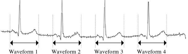
The KLT can be used on any signal that comprises a set of correlated data sequences. For example, in image processing a film sequence comprises a set of correlated images. For ECG processing, the ECG can be expressed as a set of individual ECG waveforms, which is a correlated data set, as shown in Fig.1.
Waveform 4 Waveform 2 Waveform 3
[image:2.595.112.471.178.281.2]Waveform 1
Fig. 1. Segmentation of the ECG Signal.
The KLT is the optimal transform in that:
• It completely decorrelates the original signal. (the transform coefficients are statistically independent for a Gaussian signal).
• It optimises the repacking of the signal energy, such that most of the signal energy is contained in the fewest transform coefficients.
• The total entropy of the signal is minimised.
• For any amount of compression the MSE in the reconstruction is minimised. Given these abilities, the KLT should be in widespread use. However, there are several disadvantages to using the KLT, the greatest being the computational overhead required to generate the transform vectors. The transform vectors for the KLT are the eigenvectors of the autocovariance matrix formed from the data set. To generate the KLT vectors the procedure is as follows:
1. Take N sequences (ECGs) each of L data points,
X
[ ][ ]N L . 2. Construct an average signal M[ ][ ]
M
N
X
j i j
i N
=
= −
∑
1
0 1
j
=
0
....
L
−
1
(1)3. Subtract the average signal from the original ensemble
Yi = Xi − M i=0....N −1 (2)
C
C
C
C
C
C
C
C
L
L L L L
1 1 1 2 1
2 1 2 2
1 2
, , ,
, ,
, , ,
L L
M
M
O
M
M
O
where each value Ci,j is given by
C
Y
Y
N
i j
p i p j p N ,
=
×
−
= −∑
01
1
i = 1...L, j = 1...L (3)
It is the eigenvectors of this matrix which are used as the basis vectors for the transform.
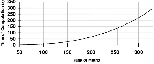
To extract the eigenvectors from a matrix of rank L, requires processing of the order
L2. It is this computation that is often quoted (refs) as being too large to be realisable, even for the relatively small values of L required for ECGs. Hence, this is why the KLT is not used, except as a benchmark for other faster schemes. However, given the computing power readily available in modern desktop PCs, this computation is no longer such a problem. Fig. 2 gives the processing time taken to extract the eigenvectors from a matrix, with rank L from 50 to 330. The algorithm used is running on a standard Pentium 200Mhz PC.
0 50 100 150 200 250 300 350
50 100 150 200 250 300
Rank of Matrix
Ti
me of Computati
[image:3.595.177.429.427.532.2]on (s)
Fig. 2. Computation Time of Eigenvectors.
based transform methods. This gives a computation time of 68 seconds and 3.1 seconds respectively to extract the eigenvectors. This is a one off computation for each recording, and so does not appear to be a great overhead. Also this time does not include the additional processing required to fill the covariance matrix, which is of order NL2.
All the eigenvectors are normalised to have unit energy, to give an orthonormal transform. The corresponding eigenvalues for these vectors show the variance distribution of the ensemble within this transform domain. This indicates how effective the repacking of the signal energy is likely to be with these vectors. Also direct study of the vectors themselves may help in the understanding the mechanisms, and component sources, present in the signal. This can help in either the preprocessing of the signal, such as to eliminate noise sources, or assist in the selection of a faster fixed transform. This is demonstrated in the results below.
3. RESULTS
Consider the signal in Fig.3.
Fig.3. Sample ECG Signal
This is a sample of a recording from the MIT-BIH arrhythmia database (recording number 101, channel 1) well known as a reference data for analyse.
If this tape is used to generate a set of transform vectors, the following results are achieved. Firstly an average waveform is generated, Fig.4, that is then subtracted from all the waveforms.
Data Point
Am
plitude
-50 0 50 100 150 200 250 300 350
0 32 64 96 128 160 192 224
Fig.4. Average Waveform
1
10
100
1000
10000
100000
0
16
32
48
64
80
96
112 128
Eigenvector Eigenvalue (log scale)
Fig.5. Eigenvalues of the Principal Eigenvectors
Vector 1. Eigenvalue = 31,825
Amplitude
-0.08 -0.06 -0.04 -0.02 0 0.02 0.04 0.06 0.08 0.1 0.12
0 64 128 192 256
Vector 2. Eigenvalue = 7232
Amplitude
-0.1 -0.05 0 0.05 0.1 0.15 0.2 0.25 0.3
0 64 128 192 256
Vector 3. Eigenvalue = 3925
Amplitude
-0.25 -0.2 -0.15 -0.1 -0.05 0 0.05 0.1
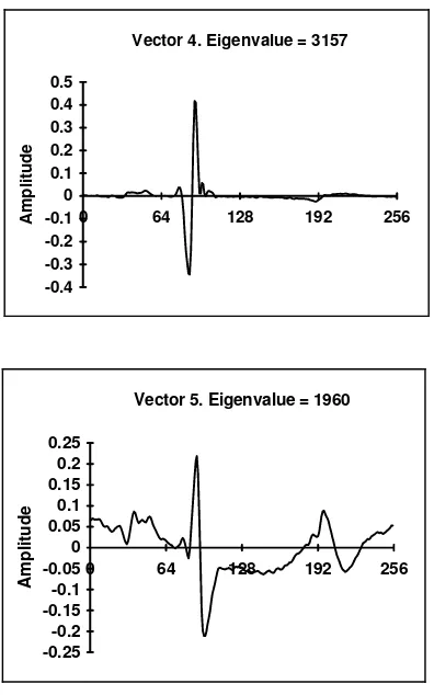
Vector 4. Eigenvalue = 3157
Amplitude
-0.4 -0.3 -0.2 -0.1 0 0.1 0.2 0.3 0.4 0.5
0 64 128 192 256
Vector 5. Eigenvalue = 1960
Amplitude
-0.25 -0.2 -0.15 -0.1 -0.05 0 0.05 0.1 0.15 0.2 0.25
[image:7.595.207.405.81.398.2]0 64 128 192 256
Fig. 6. Principal Eigenvectors
4. CONCLUSIONS
subtracting the average, vector 4 appears to be a differential of the average waveform, which suggests misalignment.
As a main conclusion is the fact that due to the apriori knowledge on the ECG waveform and its content the KL (signal dependent) transform is well suited for such data compression having an average effectiveness upon either block or time-frequency transforms.
REFERENCES
[1]. Blanco, S. Kochen, O.A. Rosso and P. Salgado, Applying time-frequency analysis to seizure EEG activity, IEEE Engineering in Medicine and Biology., January-February, 64-71, 1997.
[2]. Olkkonen, .H - Running discrete Fourier transform for time-frequency analysis of biomedical signals, Med. Eng.Phys 1995 Vol 17 pp 455-458
[3]. Philips, W - Adaptive noise removal from biomedical signals using warped polynomials, IEEE Transactions on Biomedical Engineering - May 1996 Vol- 43 NO- 5 pp- 480-492
[4]. Turbes, C.C.- Frequency and time domain studies of the micro-EEG from the brain extracellular space - Biomedical Sciences Instrumentation - 1996 Vol- 32 pp.113-118.
[5]. Fuller W,A, Introduction to statistical time series, Wiley Series in Probability and Statistics., 2 Ed., 1996.
[6]. Dripps, J. - An Introduction to time -frequency methods applied to Biomedical Signals - in Time-freq. analysis of biomed. signals IEE Colloq. Jan 1997 [7]. Pradhan, N, Dutt, DN, Sadasivan, PK, Ramesh, RG - Estimation of attractor
dimension of EEG using SVD, Sadhana-Acad. Proceedings in Engineering Sciences -Feb. 1996 Vol- 21 pp- 21-38
[8]. Martens, W. - The fast time frequency transform : a novel on -line approach to the instantaneous spectrum in Proceedings of the 14-th International Conference IEEE Eng. in med. and biology 1992 pp. 2594-2596