Full Terms & Conditions of access and use can be found at
http://www.tandfonline.com/action/journalInformation?journalCode=ubes20
Download by: [Universitas Maritim Raja Ali Haji] Date: 12 January 2016, At: 17:19
Journal of Business & Economic Statistics
ISSN: 0735-0015 (Print) 1537-2707 (Online) Journal homepage: http://www.tandfonline.com/loi/ubes20
Parametric Properties of Semi-Nonparametric
Distributions, with Applications to Option
Valuation
Ángel León, Javier Mencía & Enrique Sentana
To cite this article: Ángel León, Javier Mencía & Enrique Sentana (2009) Parametric Properties of Semi-Nonparametric Distributions, with Applications to Option Valuation, Journal of Business & Economic Statistics, 27:2, 176-192, DOI: 10.1198/jbes.2009.0013
To link to this article: http://dx.doi.org/10.1198/jbes.2009.0013
View supplementary material
Published online: 01 Jan 2012.
Submit your article to this journal
Article views: 104
View related articles
Parametric Properties of Semi-Nonparametric
Distributions, with Applications to
Option Valuation
A
´ ngel L
EO´ NDepartamento de Economı´a Financiera, Universidad de Alicante, Ap. 99, E-03080 Alicante, Spain ([email protected])
Javier M
ENCI´ABank of Spain, Alcala´ 48, E-28014 Madrid, Spain ([email protected])
Enrique S
ENTANACEMFI, Casado del Alisal 5, E-28014 Madrid, Spain ([email protected])
We derive the statistical properties of the semi-nonparametric (SNP) densities of Gallant and Nychka (1987). We show that these densities, which are always positive, are more flexible than truncated Gram– Charlier expansions with positivity restrictions. We use the SNP densities for financial derivatives val-uation. We relate real and risk-neutral measures, obtain closed-form prices for European options, and analyze the semiparametric properties of our pricing model. In an empirical application to S&P500 index options, we compare our model to the standard and Practitioner’s Black–Scholes formulas, truncated expansions, and the Generalized Beta and Variance Gamma models.
KEY WORDS: Density expansions; Gram–Charlier; Kurtosis; Skewness.
1. INTRODUCTION
In recent years, many studies have attempted to overcome the limitations of the popular normality assumption on the returns of stocks and other financial assets, which is often rejected in the empirical finance literature even after control-ling for volatility clustering effects. Although this assumption may still be reasonable if the interest focuses on the first two conditional moments (Bollerslev and Wooldridge 1992), in many financial applications, the features under study involve higher order moments such as skewness and kurtosis. An important example is option pricing theory. The Black and Scholes (1973) pricing formula, which relies on the normality of returns, remains the benchmark model due to its analytical tractability. Unfortunately, this framework is unable to capture some important puzzles, such as smiles and smirks.
However, any successful generalization of the Gaussian assumption must satisfy two crucial requirements: modeling flexibility and analytical tractability. Both needs are satisfied by the Gram–Charlier expansions introduced in option pricing theory by Jarrow and Rudd (1982), and more recently used by Corrado and Su (1996, 1997), Capelle-Blanchard, Jurczenko, and Maillet (2001), and Jurczenko, Maillet, and Negrea (2002a). As is well known, many density functions can be expressed as a possibly infinite expansion of the Gaussian density. In practice, however, the expansion is usually truncated after the fourth power, even though such truncated expansions often imply negative densities over some interval of their domain of variation, as Jondeau and Rockinger (2001) emphasize. This feature is particularly worrying in option pricing applications, because it allows for arbitrage oppor-tunities. For instance, the price of a butterfly spread with positive payoff over an interval of negative density would necessarily be negative in those circumstances. As a solution to
this problem, Jondeau and Rockinger (2001) propose to restrict the parameters of the expansion so that the density always remains positive. Unfortunately, their approach is difficult to implement even when the truncation order is low.
In this context, we propose the use of semi-nonparametric (SNP) distributions as an alternative expansion of the Gaussian density function that is always positive by construction. This distribution was introduced by Gallant and Nychka (1987) for nonparametric estimation purposes (see also Fenton and Gallant 1996; Gallant and Tauchen 1999). However, it has not been treated from a purely parametric point of view, that is, as if it reflected the actual data generating process instead of an approximating kernel. We assume that, under the real measure, asset returns follow a SNP distribution conditional on the information available at each point in time. We study first the statistical properties of this distribution, as well as its rela-tionship to the Gram–Charlier densities. Then, we combine it with an exponentially affine assumption on the stochastic dis-count factor, which enables us to transform the real measure into the risk-neutral measure required for the valuation of derivative assets, and we obtain closed-form expressions for European option prices. We also compare the SNP distributions with two other popular distributions in the option pricing lit-erature: the Generalized Beta (GB) (see Bookstaber and McDonald 1987; Liu et al. 2007, among others); and the Var-iance Gamma (VG) model of Madan and Milne (1991) and Madan, Carr, and Chang (1998). In addition, we use the Marron and Wand (1992) test suite to assess the semiparametric properties of our option pricing model when the true model is
176
2009 American Statistical Association Journal of Business & Economic Statistics April 2009, Vol. 27, No. 2 DOI 10.1198/jbes.2009.0013
not SNP. We also assess the ability of our model to fit the low-frequency smiles generated by a high-low-frequency SNP process with stochastic volatility. Furthermore, we carry out an empirical application to the S&P 500 options data of Dumas, Fleming, and Whaley (1998), in which we estimate the implied volatilities and shape parameters of our model and evaluate the performance of the SNP pricing formulas. Finally, we provide a generalized version of the SNP distribution.
The paper is structured as follows. In the next section, we study the statistical properties of SNP densities and compare them with those of Gram–Charlier expansions. In Section 3, we first relate the real and risk-neutral measures and then focus on pricing European options. Section 4 studies the semiparametric properties of our methodology, while Section 5 presents the empirical application. Finally, in Section 6, we present our gen-eralized SNP density, and provide our conclusions in Section 7. Proofs and auxiliary results can be found in the appendices.
2. DENSITY DEFINITION
We want to analyze the statistical properties of the affine transformationz¼a þbx, when the density ofxbelongs to the SNP class introduced by Gallant and Nychka (1987). Specifically, bility density function (pdf) of a standard normal random variable, and Hið Þx is the normalized Hermite polynomial of orderi. These polynomials can be defined recursively for
i$2 as
f gi2N constitutes an orthonormal basis with respect to
the weighting function fð Þx ; as illustrated by the following condition:
Z þ‘
‘
Hið ÞxHjð Þx fð Þxdx¼1ði¼jÞ
where1() is the usual indicator function. The change of var-iable formula implies that the density function ofzwill be
g zð;n;a;bÞ ¼1
where we could interpreta as a location parameter and b as a scale parameter. Note that both (1) and (3) are homogeneous of degree zero inn, which implies that there is a scale
inde-terminacy that we must solve by imposing a single normaliz-ing restriction on these parameters, such as n0 ¼ 1, or
preferably n9n¼1, which we can ensure by working with
hyperspherical coordinates (see, e.g., Fang, Kotz, and Ng 1990, Theorem 2.11).
If we expand the squared expression in (1), we can obtain the following result.
Proposition 1. Let x be an SNP random variable with densityfðx;nÞgiven by (1). Then,
ifk2Gand zero otherwise, with
G¼ k2N:jijj#k# iþj;ijþk
obtained by using the relationship between the powers ofxand the Hermite polynomials:
where the operatorEf½takes the expectation of its argument with respect to the density functionfðx;nÞin (1). Then, from
the previous noncentral moments, the corresponding central ones,mxðkÞ, can be easily obtained (e.g., Stuart and Ord 1977).
Finally, we can also compute the skewness and kurtosis coef-ficients, denoted by sk and ku, respectively. However, since m9xð Þk in (6) depends on Ef½Hið Þx
i2N, we first need to find
these moments.
Proposition 2. Letxdenote the SNP random variable with density function (1). Then, the expected value of thekth order Hermite polynomial is given by
Ef½Hkð Þx ¼gkð Þn ; ð7Þ
ifk#2m,and zero otherwise, wheregkð Þn is defined in (5).
On this basis, we can easily compute the first four non-centered moments ofxfor the important special case ofm¼2:
Lemma 1. If the density function of the random variablex
is given by (1) withm¼2, then
m9xð Þ ¼1
More generally, we can show the following:
Proposition 3. The moment generating function of the SNP density (1) is Ef½expðtxÞ ¼expðt2=2ÞLðn;tÞ, while
Sincezis an affine transformation ofx, it is trivial to find the noncentral moments of z,m9zð Þk , as a function of those ofx.
In addition, we can always choose the location and dispersion coefficientsaandbsuch thatzhas zero mean and unit variance. In particular, if we denote byz* the standardized variable
z ¼xffiffiffiffiffiffiffiffiffiffiffiffim9xð1Þ
mxð2Þ
p ; ð9Þ
then its density function can be directly obtained from (3) with
aðnÞ ¼ m9xð1Þ=pffiffiffiffiffiffiffiffiffiffiffiffimxð2Þ; bðnÞ ¼1=pffiffiffiffiffiffiffiffiffiffiffiffimxð2Þ: ð10Þ
We can also use Proposition 3 to derive the distribution of linear combinations of SNP variables. In particular, we can show that the distribution of the sum ofn iidSNP variables of order m can be expressed as a Gram–Charlier expansion of ordernmthat is always positive by construction.
Proposition 4. Define q¼Pnk¼1pkxk, where {xk}, k ¼ 1,. . .,nare iid random variables whose distribution is a SNP of ordermwith shape parametersn. Then, the distribution ofqis a Gram–Charlier expansion of order 2mnwhose density function can be expressed as
We will exploit this property to analyze the effect of time aggregation on SNP returns.
2.2 Gram–Charlier Expansion of the SNP Density
Under certain regularity conditions (see, e.g., Stuart and Ord 1977, p. 234), a density functionh yð Þcan be expressed as the product of a standard normal density times an infinite series of Hermite polynomials:
This is the so-called Gram–Charlier series of Type A. With this in mind, we will first determine the Gram–Charlier expansion of the SNP density ofz, and then we will particu-larize it for the standardized random variablez* in (9). In the case ofz, we will use the fact that, according to (3) and (4), its density can be written as
g zð ;n;a;bÞ ¼1
where Ef½ is an expectation with respect to the standard normal density. The following proposition gives a general formula for these expectations. standardized Hermite polynomial in (2) and b c rounds its argument to the nearest integer toward zero.
In consequence, the coefficients ofzdefined in (16) will be
ckðnÞ ¼
Finally, we can easily find the coefficients of the Gram– Charlier expansion of z* by substituting a and b by their respective values in (10). This expansion will generally be infinite except for one particular case. Specifically, ifn1¼n2¼
0 andm> 2, then it can be shown thatckðnÞ ¼0 fork> 2m, since aðnÞ ¼0 and bðnÞ ¼1 in that case. Lim, Martin, and
Martin (2005) have explored this restricted parametrization
withm¼4 for option pricing purposes. In this paper, though, we will not impose any restrictions on the parameters of the SNP density.
2.3 Comparison with Other Distributions
Consider a truncated Gram–Charlier expansion of the form
h zð Þ ¼þ fð Þzþ
1þX n
i¼3
ciHið Þzþ
: ð18Þ
The moments of this distribution can be obtained by using the relationships given in (6) and exploiting the orthonormality of Hermite polynomials. In this sense, notice that (18) does not include the first and second Hermite polynomials (i.e., c1 ¼ c2 ¼ 0) to ensure that this density has zero mean and unit
variance by construction. In addition, ifn¼2m, (18) involves exactly the same number of parameters as our standardized SNP variablez*. However, as Jondeau and Rockinger (2001) point out, it is necessary to impose further restrictions on the parametersci(i¼3, 4,. . .,n) to ensure that the pdf in (18) is non-negative for all values of zþ2 ð ‘;‘Þ. Unfortunately, they only determined those restrictions forn ¼4, because it becomes exceedingly difficult to find them for higher n. In contrast, we can leave the vector of parametersnfree, except
for a scale restriction, because positivity is always satisfied by a SNP density regardless of the expansion order.
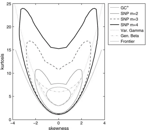
Given that bothz* andzþhave zero mean and unit variance, one may ask which of them leads to more general higher order moments. We will initially answer this question in terms of the third and fourth moments that these distributions can generate by plotting in Figure 1 the envelope of all the combinations of skewness and kurtosis form¼2, 3, and 4 andn¼4. We have used the procedure devised by Jondeau and Rockinger (2001) to obtain the frontier for a positive Gram–Charlier distribution
withn¼4, while we rely on (6) to represent the frontier of SNP densities withm¼2, 3, and 4. To allow forn0¼0, we simulate
10 million parameters n in the unit sphere and compute the
envelope of the values of skewness and kurtosis obtained from the simulated parameters. In addition, we have computed the regions of skewness and kurtosis generated by the VG dis-tribution and the log of a GB variate. Finally, we also represent the skewness-kurtosis frontier that no density function can surpass (see, e.g., Stuart and Ord 1977). The advantage of the density in (18) is that the skewness and kurtosis coefficients can be directly obtained from c3 and c4. Nevertheless, the
combinations of skewness and kurtosis that the variablezþcan generate are well within the combinations spanned by the SNP standardized variablez* with exactly the same number of free parameters, as we can see in Figure 1. For instance, whilezþ
could never be platykurtic,z* can indeed have kurtosis coef-ficients lower than 3. More importantly, the differences in minimum and maximum skewness are also substantial. Of course, by using the SNP instead of the Gram–Charlier expansion, we lose the direct interpretation of the parameters as skewness and kurtosis. However, this is also the case with many other non-Gaussian distributions, such as symmetric and asymmetric Student-t distributions, and even the GB or VG ones. Finally, it is worth recalling that the SNP distribution guarantees positive densities regardless of m. In this sense, Figure 1 shows that we could achieve much more flexibility with just one or two additional parameters. As for the other two models, we can observe that neither the GB nor the VG distributions can generate kurtosis below 3. It is also worth remarking that, although the VG can generate infinite kurtosis, it cannot yield as high a skewness as the SNP for empirically relevant levels of kurtosis. In this sense, it can be shown that the frontier of the VG is obtained when this distribution converges to a Gamma. The GB also has limited flexibility, although it allows for higher skewness than Gram–Charlier expansions once positivity restrictions are imposed. In this case, it can be shown that the upper border of its frontier is obtained when the distribution of the log of a GB variate converges to an asym-metric double exponential, which becomes a single exponential at the two points of highest absolute skewness.
To get a clearer sense of the underlying differences between the distributions of zþ and z*, we can compare the Gram– Charlier expansion of z* with (18). Since both variables are standardized, both havec0¼1 andc1¼c2¼0. The third and
fourth coefficients are functions of the skewness and kurtosis of the distributions, which we have already compared in the previous paragraph. Still, the main difference betweenz* and
zþ is found in the higher order coefficients. In particular, whereas (18) imposes thatck¼0 for allk>n, such a restriction no longer holds forz*.
3. OPTION VALUATION 3.1 From the Real to the Risk-Neutral Measure,
and Vice Versa
Consider a frictionless market with a risk-free asset and a risky asset with priceStat timet. For anyT>t, we can always expressSTin terms ofStunder the real measurePas
Figure 1. Regions of skewness and kurtosis. Note: GCþdenotes a Gram–Charlier expansion of ordern¼4 with positivity restrictions, while Gen. Beta denotes the distribution of the log of a Generalized Beta.
ST [ Stexp mts unit variance conditional on the information available at timet. In this context,mtandst, which in general will be functions of the information known att, represent the conditional mean and volatility per unit of time of log (ST/St). In what follows, we will assume that z ¼að Þ þnt bð Þnt xP, whereað Þnt and bð Þnt are
defined in (10), andxPis an SNP variate with shape parameters
nt. With this notation, we can write the log-return asyT¼log
Our solution to the option pricing problem will be based on the use of a stochastic discount factor with an exponential affine form:
Mt;T¼expðatyTþbttÞ: ð20Þ
where again at and bt can be functions of the information known at time t. Such a specification corresponds to the Esscher transform used in insurance (Esscher 1932). In option pricing applications, this approach was pioneered by Gerber and Shiu (1994), and has also been followed by Buhlman et al. (1996, 1998), Gourieroux and Monfort (2006, 2007), and Bertholon, Monfort, and Pegoraro (2003), among others. The following result provides the conditions for absence of arbitrage.
Proposition 6. Let rt be the risk-free rate and It the in-formation set at time t. If the conditional distribution of the log-return of the risky asset is an SNP of order m, then the stochastic discount factor (20) satisfies the arbitrage-free conditions
From these two constraints, we can easily express bt as a function ofat. Hence,atcan be obtained by solving a single nonlinear equation, which is an implicit function of the remaining parameters of the model.
In this context, ifQdenotes the risk-neutral measure whose numeraire is the risk-free asset, the real and risk-neutral mea-sures can be easily related by means of the Radon–Nykodym derivative, which in this case is proportional to the discount factor
expðrttÞ, so that the discount factor correctly prices the
risk-free asset. As a result, we can obtain the risk-neutral density from (24) as
fQðyTjItÞ ¼expðrttÞMt;TfPðyTjItÞ: ð25Þ
On this basis, we can fully characterize the risk-neutral measure as follows.
Proposition 7. If the asset priceSTis given by (19) under the real measureP, where the conditional distribution of its log--return betweentandTis a SNP of order m with shape param-etersnt, then it can be written under the risk-neutral measureQ
as
andk*is a standardized SNP variable of order m with shape parametersut ¼ ðu0t;u1t;. . .;umtÞ0;such that
Therefore, in a SNP context, the change of measure affects not only the mean and the variance of the log price, but also the higher moments, as can be seen from the differences between
utandnt. For the case ofm¼2, for instance, we can show that note that the SNP distribution is shared by the real and risk-neutral measures. Also, it is important to emphasize that this change of measure is always feasible, because there are no restrictions on the shape parameters of the SNP distribution. Our results can be extended to more complicated specifications of the stochastic discount factor. For instance, an exponential quadratic form would also yield an SNP distribution of the same order under the risk-neutral distribution (the details are available upon request). In those cases, though, we would need to consider a larger number of assets to identify the parameters of the pricing kernel.
Obviously, our framework also allows us to value derivative assets by focusing on the risk-neutral measure directly without any reference to its relationship with the real measure, as in Jondeau and Rockinger (2001) or Jurczenko, Maillet, and Negrea (2002a,b). To follow this second approach, we just have to regardut,mQt , andsQt as the structural parameters. The
fol-lowing proposition gives the expression that the risk-neutral drift must have to satisfy the martingale restriction (Longstaff 1995).
Proposition 8. If asset priceSTis given by (26) under the risk-neutral measureQ, where the conditional distribution of its log-return betweentandTis an SNP of ordermwith shape parameters ut, then the drift mQt will satisfy the martingale
restriction if and only if
mQt ¼rt ð1=tÞlogLðut;lQtÞ
Not surprisingly, we show in Appendix C (available as on online supplement) that (27) and (30) coincide, which confirms that both strategies are indeed equivalent. This equivalence result has important computational advantages in empirical applications such as ours that only use option price data, because it allows one to estimate the option values from the risk-neutral parameters without having to solve the nonlinear equations (22) and (23) within the optimization algorithm. At the same time, if we had data on the underlying, we could obtain the implied real-measure parameters. In particular, for a given driftmt, risk-free ratert, and risk-neutral parameterss
Q
t
andut, we can recover the parameters of the real measurest
andnt, together with the coefficient of relative risk aversionat,
from the following system of equations:
mts
count factorbtcan be obtained from either (22) or (23).
3.2 Option Pricing
LetCtbe the value at timetof a European call option with strike priceK and expiration at timeT, and let Stdenote the underlying asset value. We can expressCtas
Ct¼expðrttÞEQ ðSTKÞþ conditional nature of (32), which implies that all the parameters of the model can potentially depend on the information avail-able at timet. If we define the regionA¼{ST >K}, we can rewrite (32) as
Ct¼expðrttÞEQ½ST1ðAÞjIt
KexpðrttÞEQ½1ðAÞjIt:
ð33Þ
Following Geman, Karouri, and Rochet (1995), we can further simplify the calculations by changing the numeraire to the ratio of the risky asset pricesST/St, which gives an alter-native risk-neutral measure Q1. Then, if we use the Radon–
Nikodym derivative,
we can easily express any expectation underQin terms ofQ1.
Specifically, we will have
which, once introduced in (33), gives us the general formula,
Ct¼StEQ1½1ðAÞjIt KexpðrttÞEQ½1ðAÞjIt
¼StPrQ1½ST>KjIt KexpðrttÞPrQ½ST>KjIt: ð35Þ
The analytical tractability of the SNP distribution allows us to obtain closed form expressions for the probabilities in (35):
Proposition 9. The price at timetof a European call option with strikeKwritten on the stockSTdefined by (26) under the risk-neutral measure can be expressed as
CtSNP¼StPrQ1½x>dtjIt
andF() is the cumulative distribution function of the standard normal density.
As expected, (36) reduces to the Black and Scholes (1973) formula whenu0t¼1 andukt¼0"k$1. Importantly, if we treat the coefficientsgkof the Gram–Charlier expansion (4) as shape parameters themselves, instead of functions of eitherntorut, we
can show that (36) is also valid when the distribution of the underlying asset return is a finite Gram–Charlier expansion. As a consequence, we can use Proposition 9 to obtain closed form option prices when returns follow a high-frequency process with iid SNP innovations, since Proposition 4 shows that their dis-tribution at low frequencies is a Gram–Charlier expansion.
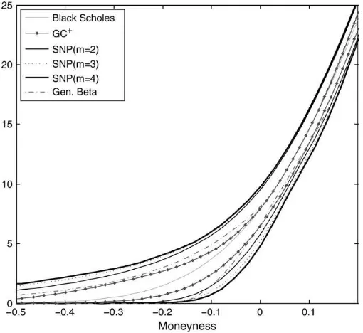
In Figure 2, we compare the range of call prices that the SNP density can produce with the corresponding ranges obtained for the Gram–Charlier expansion with positivity restrictions and the GB model. Not surprisingly, the higher flexibility of the SNP in modeling skewness and kurtosis that we saw in Figure 1 results in a wider range of call prices. The only exception is the VG model, which can reach the arbitrage bounds, but only under the limiting case in which the underlying distribution converges to a Bernoulli whose skewness tends to 6‘.
Importantly, a larger value ofmalso leads to an SNP with even
broader range. Nevertheless, there is a close relationship between the different pricing models: the Gram–Charlier call price formula can be obtained as a fourth-order Taylor expansion of (36), while the Black–Scholes formula corre-sponds to a second-order one (see Appendix A for further details).
4. SEMIPARAMETRIC PROPERTIES OF THE SNP OPTION PRICING MODEL
4.1 Estimation with a Misspecified Model
Fenton and Gallant (1996) and Gallant and Tauchen (1999) used the Marron and Wand (1992) test suite to analyze the semiparametric properties of SNP distributions in density estimation and in the implementation of the Efficient Method of Moments, respectively. However, their semiparametric properties in option pricing applications have not been studied. In this section, we will assess the performance of our option pricing model when the true distribution is not SNP.
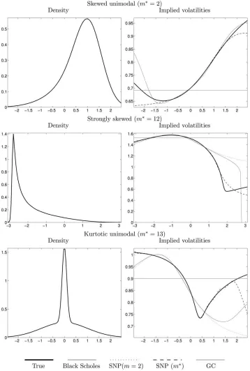
Specifically, we will assume that the true distribution of the underlying asset return is one of the first nine non-Gaussian dis-tributions proposed by Marron and Wand (1992). For each of them, we generate 1,000 call option prices from the true model, with a range of moneyness uniformly distributed between 63 times the standard deviation of the underlying asset return. Finally, we estimate the parameters of the following misspecified models by minimizing the root-mean-square pricing errors (RMSEs): Black–Scholes, Gram–Charlier with two shape parameters, SNP withm¼2, and SNP of orderm* such that the RMSE divided by the mean option price is less than 10 basis points.
Some selected results are displayed in Figure 3. The left panels show the shape of the true density, whereas the right
panels display the true implied volatilities together with the ones estimated with the misspecified models. Since none of these models is Gaussian, Black–Scholes performs poorly in most cases. The models with two shape parameters perform reasonably well in some examples, such as the skewed and kurtotic unimodal cases. However, in some other examples, such as the strongly skewed, the Gram–Charlier parameter estimates cannot guarantee the positivity of the density. The consequence is that Gram–Charlier implied volatilities sud-denly jump to zero for some ranges of the moneyness. In contrast, our pricing model does not suffer from this restriction. Of course, if we letm !‘, then we will be able to exactly reproduce all the volatility smiles. However, we are able to show that even for finite m, the SNP already performs very well. In this sense, we can check that we obtain substantial im-provements in fit in all cases as we increase the order of the SNP.
4.2 Temporal Aggregation
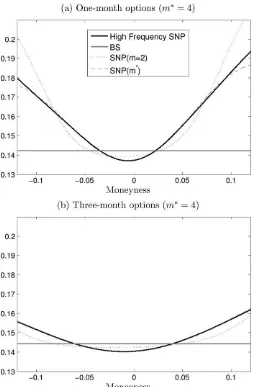
From Proposition 4, we know that the distribution of aggregated SNP returns is not an SNP of the same order, not even when they are iid. In this subsection, we assess the ability of our model applied to low-frequency data to fit option prices that have been generated with a high-frequency process with SNP returns. To do so, we model the weekly process of log-returns with a non-iid SNP distribution of orderm¼2, whose volatility follows a persistent binary Markov chain. The skewness and kurtosis of this process conditional on the vola-tilities of the two states that we consider are characterized by the shape parameters of the SNP distribution, while the prob-abilities of remaining in each of these states determine the unconditional variance and the persistence of the stochastic volatility. All these parameters have been calibrated using S&P 500 weekly return data from 1950 to 2006. Although for the purposes of our exercise we could have considered a con-tinuous distribution for volatility, we have chosen a Markov chain only because we can obtain closed form option prices. Specifically, we consider every possible volatility path that the Markov chain can generate. Along any of those paths, Propo-sition 4 implies that the distribution of the log-return between the initial and final dates is just a Gram–Charlier expansion, for which Proposition 9 applies if we impose (30) to ensure that the martingale restriction is satisfied. Finally, we can express the call price as a weighted sum of the option prices in each pos-sible path, with weights that correspond to their unconditional probabilities of occurring. We have generated from this process 1,000 option prices maturing in one and three months with the same range of moneyness as in the previous subsection. We fit SNPs of increasing order to these prices until the RMSE divided by the mean option price is less than 10 basis points.
As shown in Figure 4, an SNP withm¼4 is enough to yield a RMSE below our target for both maturities. This is somewhat surprising if we take into account that, for a given volatility path, the distributions of the one and three month log-returns are Gram–Charlier expansions of order 16 and 48, respectively (Proposition 4). Thus, we believe that the time incoherence problem should not be an issue of major concern in our context. We can also notice in Figure 4 the flattening of the smile at the
Figure 2. Flexibility to model departures from Black–Scholes. Note: This figure shows the minimum and maximum European call prices that each distribution can yield for a strike price of 100, a maturity of 3 months, and a risk-free interest rate of 3%. GCþdenotes a Gram– Charlier expansion of ordern¼4 with positivity restrictions.
longer horizon, which is consistent with the empirical evidence (see, e.g., Das and Sundaram 1999).
5. EMPIRICAL PERFORMANCE OF SNP OPTION PRICING
In this section, we apply the SNP option valuation Equation (36) in Proposition 9 to S&P 500 index options using the same database as Dumas, Fleming, and Whaley (1998). Option
pri-ces were collected every Wednesday between 2:45 p.m. and 3:45 p.m. from June 1988 to December 1993, which makes a total number of 292 days. Options are European style and expire on the third Friday of each contract month. We will focus on call options, and use the bid-ask midprice for esti-mation purposes. The riskless interest rate will be proxied by the T-bill rate implied by the average of the bid and ask discounts reported in theWall Street Journal. To account for the presence
Figure 3. Estimation of options from Marron–Wand test suite. Notes: Marron–Wand densities are represented in the left panels. The cor-responding true implied volatilities are plotted on the right panels, together with the ones obtained by estimating the SNP and Gram–Charlier option pricing models. SNP (m*) denotes the SNP model of lowest order that makes the RMSE divided by the mean call price smaller than 10 basis points. The remaining non-Gaussian models only use two shape parameters.
of dividends, the implied forward price is computed as the current stock priceStminus the present value of dividendsDt times the interest accrued until maturity; i.e., Ft;T¼ ðSt
DtÞexpðrttÞ (Dumas, Fleming, and Whaley 1998 provides
further details).
We will compare the performance of the SNP option valu-ation framework with the following competing models: the standard Black and Scholes (1973) model, the Gram–Charlier expansion with positivity restrictions, the GB and VG models, and finally a variant of the Black–Scholes model, where the volatility is assumed to be a quadratic function of moneyness. We will call this methodology Practitioners’ Black–Scholes, a name inspired by its wide use in the financial industry. To guarantee positivity, we will consider the parametrization
sð Þ ¼x r0þr1ðxr2Þ 2
ð38Þ
wherer0> 0,r1$0, andx¼Ft,T/K. Finally, note that, since we are using implied forward prices, an adjustment in the spirit of Black (1976) is needed in all cases.
We consider separate estimations for short and long matur-ities. Specifically, we estimate the implied volatility and the remaining shape parameters of each model by minimizing the sum of squared pricing errors between the observed option prices and the ones implied by the models. To select the short maturity group, we begin by considering call options that mature in 45 days for the first day in the sample. We track those options every week until two weeks before they expire. Then, we move to the next group of options that are 45 days away from expiration and start the tracking process again. At the end, we have data on 3,462 call option prices, with median time to expiration of 24 days, and a number of options per day that ranges from 4 to 25, with a median of 11. In the long maturity group, we follow an analogous selection process. In particular, we have selected 4,306 call option prices with a median time to maturity of 150 days. The number of prices per day also ranges between 4 and 25, but the median is now 15. Our empirical results are essentially unaffected by conditioning our estima-tion procedure on having at least six or seven opestima-tions per day. The main reason is that only 11 (10) out of the 292 days in our database have less than 6 options available across strikes for the short (long) maturity group.
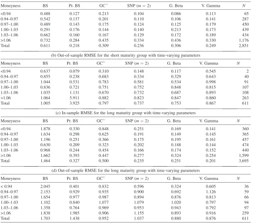
Tables 1a–1d report the RMSEs of the six competing models when we allow all the parameters of the conditional dis-tribution of returns to vary each Wednesday, which is consistent with the conditional nature of our pricing framework. We also provide information on the degree of fit achieved for different degrees of moneyness using the six categories proposed by Bakshi, Cao, and Chen (1997), together with the number of options in each category. Tables 1a and 1c report in-sample RMSEs based on the first four years of data. In contrast, Tables 1b and 1d report out-of-sample results based on pricing errors for each Wednesday in the last year of the sample using the parameters estimated on the previous Wednesday. In the short maturity group, Practitioners’s Black–Scholes and the SNP are the two best performing models in-sample, followed by the VG and GB models. However, if we look at the out-of-sample results, we can observe that Practitioner’s Black– Scholes shows a strong parameter instability, whereas the other three models are much more stable. In the long maturity group, again, the SNP, GB, and VG models yield the lowest RMSEs, although VG yields a slightly better fit in this case. Nevertheless, the differences between these three models are very small, whereas the RMSEs of the Black–Scholes, Gram– Charlier with positivity restrictions, and Practitioners’ Black– Scholes models are clearly higher.
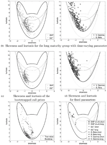
In Figures 5a and 5b, we have plotted the skewness and kurtosis values implied by the SNP, Gram–Charlier with pos-itivity restrictions, and GB and VG models for each day in the in-sample period. Several important patterns arise from these figures. First, there is high dispersion in the estimated higher order moments, although skewness is usually negative and kurtosis is typically higher than 3. Second, skewness and kur-tosis tend to be lower when the time to expiration is longer.
Figure 4. Fit of the implied volatility of a multiperiod SNP process. Notes: SNP (m*) denotes the SNP model of lowest order that makes the RMSE divided by the mean call price smaller than 10 basis points. The option prices of the high-frequency SNP model have been gen-erated by assuming that the weekly log-returns under the risk-neutral measure are SNP of order 2 whose skewness and kurtosis are0.4 and 6.5, respectively. Finally, the volatility follows a Markov chain with two states: s1 ¼ 0.1960 and s2 ¼ 0.1023. The probabilities of
remaining in states 1 and 2 arep¼0.9787 andq¼0.9847, respec-tively. The risk-free rate is set atr¼3%.
Furthermore, skewness and kurtosis in Gram–Charlier den-sities with positivity restrictions are usually on the frontier of values compatible with these densities. This is also observed with the VG and especially with the GB model. In particular, market prices often suggest a more (negative) skewness than these models are able to account for. However, some SNP estimates are also located on the frontier, especially in the short maturity group. Although we could easily enlarge the SNP frontier by simply increasing the order m (Figure 1), it is interesting to analyze in more detail the possible sources of the high sampling variability.
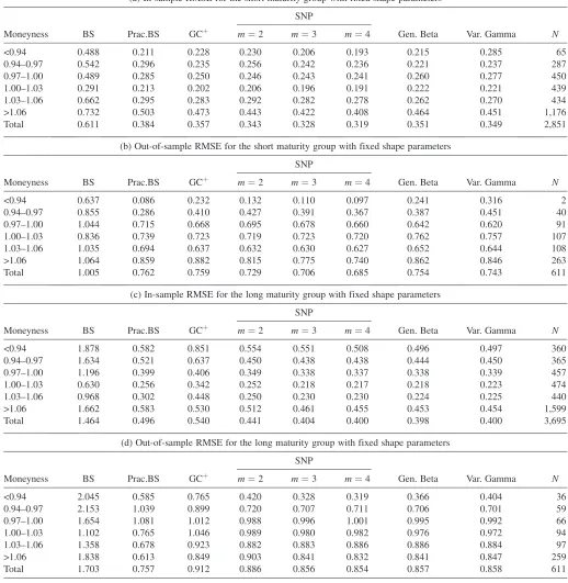
To do so, we have carried out the following bootstrap exercise. First, we group the SNP pricing errors obtained for short
maturities in the six moneyness categories already considered. Then, we simulate prices for a specific but broadly representa-tive day (November 13, 1991), by adding random pricing errors to the 19 prices of that day estimated with the SNP model. In this sense, we sample the errors that we add to each price from the same moneyness category to which that price belongs. In this way, we take into account possible distributional differences between pricing errors for, say, deep in-the-money and out-of-the-money options. Finally, we re-estimate the SNP model on the simulated data. We plot the implied skewness and kurtosis for 1,000 such simulations in Figure 5c. As we can observe, the estimates are again highly disperse and basically cover the entire region of negative skewness. Nevertheless, the true option prices
Table 1
(a) In-sample RMSE for the short maturity group with time-varying parameters
Moneyness BS Pr. BS GCþ SNP (m¼2) G. Beta V. Gamma N
<0.94 0.488 0.127 0.213 0.104 0.086 0.113 65
0.94–0.97 0.542 0.137 0.201 0.110 0.106 0.141 287
0.97–1.00 0.489 0.143 0.175 0.124 0.125 0.179 450
1.00–1.03 0.291 0.176 0.144 0.140 0.213 0.173 439
1.03–1.06 0.662 0.160 0.167 0.129 0.172 0.189 434
>1.06 0.732 0.284 0.435 0.334 0.436 0.330 1,176
Total 0.611 0.218 0.309 0.236 0.306 0.249 2,851
(b) Out-of-sample RMSE for the short maturity group with time-varying parameters
Moneyness BS Pr. BS GCþ SNP (m¼2) G. Beta V. Gamma N
<0.94 0.637 0.079 0.310 0.148 0.117 0.545 2
0.94–0.97 0.855 0.238 0.683 0.334 0.329 0.643 40
0.97–1.00 1.044 0.531 0.783 0.581 0.534 0.998 91
1.00–1.03 0.836 0.721 0.751 0.752 0.848 0.815 107
1.03–1.06 1.035 1.131 0.670 0.732 0.687 0.893 108
>1.06 1.064 5.911 0.882 0.823 0.847 0.860 263
Total 1.005 3.925 0.797 0.737 0.753 0.867 611
(c) In-sample RMSE for the long maturity group with time-varying parameters
Moneyness BS Pr. BS GCþ SNP (m¼2) G. Beta V. Gamma N
<0.94 1.878 0.330 0.848 0.251 0.169 0.141 360
0.94–0.97 1.634 0.298 0.625 0.191 0.149 0.145 365
0.97–1.00 1.196 0.251 0.366 0.175 0.195 0.161 457
1.00–1.03 0.630 0.209 0.323 0.202 0.188 0.144 474
1.03–1.06 0.968 0.244 0.454 0.166 0.174 0.152 440
>1.06 1.662 0.393 0.447 0.277 0.324 0.254 1,599
Total 1.464 0.327 0.500 0.235 0.251 0.201 3,695
(d) Out-of-sample RMSE for the long maturity group with time-varying parameters
Moneyness BS Pr. BS GCþ SNP (m¼2) G. Beta V. Gamma N
< 0.94 2.045 0.401 0.832 0.596 0.324 0.605 36
0.94–0.97 2.153 0.929 0.935 0.900 0.692 1.126 59
0.97–1.00 1.654 0.977 0.987 0.894 0.876 0.813 66
1.00–1.03 1.102 0.840 1.077 1.079 1.020 0.797 94
1.03–1.06 1.358 0.764 0.969 0.953 0.943 0.792 97
>1.06 1.838 1.985 0.906 1.155 0.893 0.916 259
Total 1.703 1.438 0.952 1.037 0.880 0.876 611
NOTES: In-sample analysis uses different parameters for each Wednesday from 1988 to 1992, while out-of-sample tables use the parameters estimated on the previous Wednesday during 1993. Moneyness is defined as the ratio of the implicit forward price of the underlying asset to the strike price. BS, Pr. BS, GCþ, G. Beta, and V. Gamma denote, respectively, Black–Scholes, Practitioners’ Black–Scholes, Gram–Charlier with positivity restrictions, and Generalized Beta and Variance Gamma models.Ndenotes the number of option prices per moneyness category.
have constant parameters by construction, which approximately correspond to skewness of1.5 and kurtosis of 7.7 (Figure 5c).
Therefore, it may well be the case that even if the true parameters are constant, the high variation in skewness and kurtosis that we observe in Figures 5a and 5b simply results from the relatively low number of prices with which we are estimating the daily models. For that reason, we also study the performance of all the different models under the assumption that the conditional distribution of standardized log-returns (or r1 and r2 in (38)) is time invariant, while volatility (or the
intercept r0 in Practitioner’s Black–Scholes) is allowed to
change over time as before. Again, we carry out in-sample and out-of-sample analyses, which show that the SNP, GB, and VG models perform more or less on the same level, while the remaining models yield less satisfactory results (see Tables 2a–2d). We can also note that, by increasing the order of the SNP, we can improve its performance without deteriorating its out-of-sample stability.
If we compare the SNP pricing errors in Tables 2b and 2d with those of Tables 1b and 1d, we can observe that the
Figure 5. Skewness and kurtosis. Notes: The results in Figures 5a and 5b correspond to separate estimations for each Wednesday in-sample, while to obtain Figure 5d, all parameters except volatility are assumed to be constant over the entire sample. In Figures 5a and 5b, SNP refers to a SNP distribution of order 2. GCþ, G. Beta, and V. Gamma denote, respectively, the Gram–Charlier expansion (n¼4) with positivity restrictions and the Generalized Beta and Variance Gamma models, while ‘‘Short’’ and ‘‘Long’’ denote the short and long maturity groups.
assumption of constant shape parameters does indeed yield better out-of-sample results. Importantly, the SNP with fixed parameters generally performs better out-of-sample than the remaining models with time varying parameters. In terms of skewness and kurtosis, Figure 5d shows that SNP estimations are no longer at the frontier. In contrast, Gram–Charlier and GB estimates are very close to or exactly on their respective frontiers.
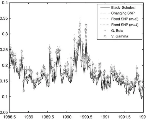
As a sanity check, Figure 6 confirms that the main differ-ences between Black–Scholes and the remaining non-Gaussian models lie in the tails of the distributions, and not so much in the temporal evolution of the option-implied volatilities.
Another interesting issue is whether the main reason for the rejection of the Black–Scholes model is skewness or excess kurtosis. To find out, we have re-estimated our SNP model for
m¼2 with fixed parameters imposing zero skewness first, and
Table 2
(a) In-sample RMSE for the short maturity group with fixed shape parameters
Moneyness BS Prac.BS GCþ
SNP
Gen. Beta Var. Gamma N
m¼2 m¼3 m¼4
<0.94 0.488 0.211 0.228 0.230 0.206 0.193 0.215 0.285 65
0.94–0.97 0.542 0.296 0.235 0.256 0.242 0.236 0.221 0.237 287
0.97–1.00 0.489 0.285 0.250 0.246 0.243 0.241 0.260 0.277 450
1.00–1.03 0.291 0.213 0.202 0.206 0.196 0.191 0.222 0.221 439
1.03–1.06 0.662 0.295 0.283 0.292 0.282 0.278 0.262 0.270 434
>1.06 0.732 0.503 0.473 0.443 0.422 0.408 0.464 0.451 1,176
Total 0.611 0.384 0.357 0.343 0.328 0.319 0.351 0.349 2,851
(b) Out-of-sample RMSE for the short maturity group with fixed shape parameters
Moneyness BS Prac.BS GCþ
SNP
Gen. Beta Var. Gamma N
m¼2 m¼3 m¼4
<0.94 0.637 0.086 0.232 0.132 0.110 0.097 0.241 0.316 2
0.94–0.97 0.855 0.286 0.410 0.427 0.391 0.367 0.387 0.451 40
0.97–1.00 1.044 0.715 0.668 0.695 0.678 0.660 0.642 0.620 91
1.00–1.03 0.836 0.739 0.723 0.719 0.723 0.720 0.762 0.757 107
1.03–1.06 1.035 0.694 0.637 0.632 0.630 0.627 0.652 0.644 108
>1.06 1.064 0.859 0.882 0.815 0.775 0.740 0.862 0.846 263
Total 1.005 0.762 0.759 0.729 0.706 0.685 0.754 0.743 611
(c) In-sample RMSE for the long maturity group with fixed shape parameters
Moneyness BS Prac.BS GCþ
SNP
Gen. Beta Var. Gamma N
m¼2 m¼3 m¼4
<0.94 1.878 0.582 0.851 0.554 0.551 0.508 0.496 0.497 360
0.94–0.97 1.634 0.521 0.637 0.450 0.438 0.438 0.444 0.450 365
0.97–1.00 1.196 0.399 0.406 0.349 0.338 0.337 0.338 0.339 457
1.00–1.03 0.630 0.256 0.342 0.252 0.218 0.217 0.218 0.223 474
1.03–1.06 0.968 0.302 0.448 0.250 0.230 0.230 0.224 0.225 440
>1.06 1.662 0.583 0.530 0.512 0.461 0.455 0.453 0.454 1,599
Total 1.464 0.496 0.540 0.441 0.404 0.400 0.398 0.400 3,695
(d) Out-of-sample RMSE for the long maturity group with fixed shape parameters
Moneyness BS Prac.BS GCþ
SNP
Gen. Beta Var. Gamma N
m¼2 m¼3 m¼4
<0.94 2.045 0.585 0.765 0.420 0.328 0.319 0.366 0.404 36
0.94–0.97 2.153 1.039 0.899 0.720 0.707 0.711 0.706 0.701 59
0.97–1.00 1.654 1.081 1.012 0.988 0.996 1.001 0.995 0.992 66
1.00–1.03 1.102 0.765 1.046 0.989 0.980 0.982 0.976 0.972 94
1.03–1.06 1.358 0.678 0.923 0.882 0.883 0.886 0.886 0.884 97
>1.06 1.838 0.613 0.849 0.903 0.841 0.832 0.841 0.847 259
Total 1.703 0.757 0.912 0.886 0.856 0.854 0.857 0.858 611
Notes: In-sample analysis (1988–1992) allows volatility to be time varying, but the other shape parameters are kept fixed. Out-of-sample estimates (1993) use for each week the volatility from the previous week and the fixed shape parameters estimated from the first five years. Moneyness is the ratio of the implicit forward price to the strike price. BS, Pr. BS, GCþ, G. Beta, and V. Gamma denote, respectively, Black–Scholes, Practitioners’ Black–Scholes, Gram–Charlier with positivity restrictions, and Generalized Beta and Variance Gamma models.Ndenotes the number of option prices per moneyness category.
then kurtosis equal to 3. Interestingly, it turns out that, when we force the skewness to be zero, we obtain the Black–Scholes special case. In contrast, if we fix the kurtosis to 3, we obtain substantial negative skewness for both the short and long maturity groups. Hence, it seems that negative skewness plays a more fundamental role in determining option prices than does excess kurtosis. This result is likely to be related to the specific features of equity index options, which are typically charac-terized by significant smirks rather than purely symmetric smiles, especially after the 1987 stock market crash (see, e.g., Brown and Jackwerth 2004). However, it is beyond the scope of this paper to assess whether this result is specific to the equity-index market.
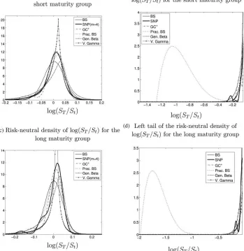
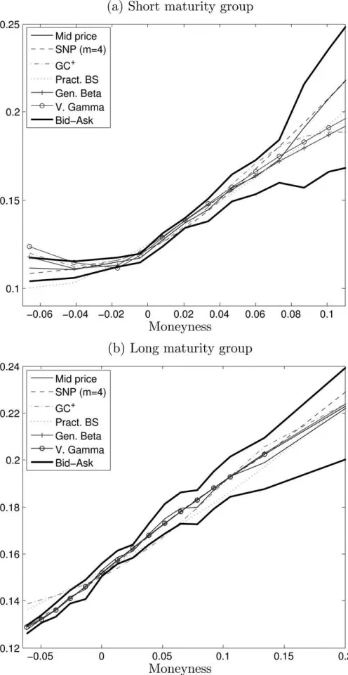
Finally, we compare the estimated conditional risk-neutral densities in Figures 7a to 7d for the same day as in the bootstrap exercise, having obtained the density implied by the Practi-tioner’s Black–Scholes model from the second derivative of the call price with respect to the strike (Breeden and Litzenberger 1978). All the models except Black–Scholes imply negatively skewed and peaked densities, but they are reasonably similar at the center, except for the much higher peaks in the VG den-sities. In fact, it turns out that this density has a pole near zero for the long maturity group. However, zooms of the left tails show that the Practitioner’s Black–Scholes model attaches unreasonably high probabilities to extreme negative events. This result is consistent with the fact that the Practitioner’s Black–Scholes method gives relatively good results in-sample but unrealistic implications for out-of-the-money calls. In Figure 8, we compare the smiles that each model can generate with the bid, ask, and midprice quotes for our chosen repre-sentative day. This figure shows a highly asymmetric smile, which Practitioner’s Black–Scholes tries to fit with quadratic curve, at the cost of not providing very reliable results at the extremes (in particular, the out-of-the money area). This pic-ture also shows that the rather limited amount of skewness
allowed by ‘‘positive’’ Gram–Charlier densities prevents them from reproducing the empirical smile as we get deeper in the money. However, lack of liquidity is stronger in deep in-the-money options, so the real importance of this result must be taken with some caution.
6. EXTENSIONS
The SNP density of ordermis constructed by multiplying the Gaussian density by a squared polynomial of orderm. The fact that the polynomial of the expansion is a perfect square is a sufficient but not necessary condition for positivity of the final density. Hence, we can create a generalized SNP (GSNP) density by multiplying the Gaussian density with an otherwise unrestricted positive polynomial P2m(x) of order 2m. This distribution will include as particular cases both the SNP and the Gram–Charlier density with positivity restrictions.
The positivity ofP2m(x) is ensured if its roots are either real and double, or complex conjugates. In contrast, in the SNP case, the complex roots must always be double. Meddahi (2001) shows that a necessary and sufficient condition for
P2m(x) to be positive is that it can be written as the sum of two squared polynomials of orderm.
Interestingly, we can interpret the GSNP density as a mixture of two SNP densities with the same location and scale:
Proposition 10. The GSNP density can be written as
fGSNPðx;n1;n2Þ ¼pðn1;n2Þfðx;n1Þ þ ½1pðn1;n2Þfðx;n2Þ;
where n1 and n2 are vectors of dimension m and m 1, respectively,f(x;n1) is defined in (1), and
pðn1;n2Þ ¼ n91n1 n91n1þn92n2:
This interpretation can be exploited to extend the results of the paper to this generalized class of distributions. Nevertheless, despite the increased generality of the GSNP, we have found that it does not seem to provide a higher flexibility in terms of skewness, kurtosis, or range of option prices than a standard SNP density of the same order. A more thorough study of the char-acteristics of the GSNP density is left for future research.
7. CONCLUSIONS
The SNP distribution was introduced by Gallant and Nychka (1987) for nonparametric estimation purposes. In contrast, we propose to use it as a parametric model. This distribution shares the analytical tractability of truncated Gram–Charlier expansions, but its density is always positive.
We obtain its moments, show its flexibility in terms of skewness and kurtosis, and derive the distribution of linear combinations. Next, we focus our attention on option pricing, and show that, if the log of the underlying asset price has a conditional SNP distribution under the real measure, and the stochastic discount factor is exponentially affine, then the log of the underlying asset price will also have a conditional SNP distribution of the same order under the risk-neutral measure. On this basis, we obtain closed form expressions for European option prices. We also show that our SNP option pricing formula
Figure 6. Option-implied volatilities for the short maturities Note: ‘‘Fixed SNP’’ assumes that the shape parameters of the SNP are constant over time, while ‘‘Changing SNP’’ allows them to be time varying. Gen. Beta and V. Gamma denote, respectively, the General-ized Beta and Variance Gamma models.
can approximate arbitrarily well the prices of options whose true densities are not SNP. Furthermore, we apply our pricing formulas to obtain exact option prices in a high-frequency SNP model. In this sense, we show that a low-order SNP can approximate very well the behavior of low-frequency option prices generated by a stochastic volatility high-frequency proc-ess with SNP innovations.
Finally, we carry out an empirical application to the S&P 500 options data of Dumas, Fleming, and Whaley (1998). We compare the performance of our pricing formulas with the Black and Scholes (1973) model, the Practitioner’s Black– Scholes procedure, the Gram–Charlier density with positivity restrictions, and the GB and VG models. We estimate the shape parameters and the implied volatility that minimize the sum of squared pricing errors of these models. We find that the SNP, together with the GB and the VG, are the best performing models, both in-sample and out-of-sample. We also find a high dispersion in the daily estimates of skewness and kurtosis, which is probably due to sampling variability. In this sense, we find that the pricing performance of our model improves
out-of-sample if we keep the shape parameters constant over time. It is also worth mentioning that skewness seems to be relatively more important than excess kurtosis for the empirical rejection of the Black–Scholes model. This result is probably due to the asymmetric smiles that are typically observed for equity index options.
We propose a generalized version of the SNP distribution that nests all positive Gram–Charlier expansions. We show that it can be generated as a mixture of two SNP variables with the same location and scale, which allows us to extend our previous results to this density.
A fruitful avenue for future research would be to exploit the relationship between real and risk-neutral measures in the estimation of our option pricing model by combining data on the underlying asset price, which is informative about the real measure, with option price data, which contains information about the risk-neutral measure (Jackwerth 2000). It would also be interesting to explore possible time varying specifications for the parameters of the model, such as GARCH parametrizations for the volatility (Heston and Nandi 2000), and analogous
Figure 7. Risk neutral densities. Notes: These results are based on the volatility estimated on November 13, 1991, but the shape parameters are estimated using data between 1988 and 1992. Pract. BS denotes a model in which volatility is a quadratic function of moneyness. SNP refers to a SNP distribution of order 4, while GCþ, Gen. Beta, and V. Gamma denote, respectively, the Gram–Charlier distribution (n¼4) with positivity restrictions and the Generalized Beta and Variance Gamma models.
extensions for the remaining shape parameters, as in Hansen (1994) or Jondeau and Rockinger (2005). Similarly, it would also be worth exploring the flexibility of the SNP and gener-alized SNP distributions for risk-management purposes.
APPENDIX: A RELATIONSHIP WITH GRAM–CHARLIER OPTION PRICING MODELS
We can express (36) in terms of the infinite Gram–Charlier expansion of the SNP distribution as follows.
Proposition 11. The call price CSNPt in (36) can be re-written in terms of an infinite expansionCSNPt ¼j0tþj3tsktþ
in (26), is regarded as a function of the standardized random variablek*, while the coefficientsck(ut) are given in (17).
We can use Proposition 11 to relate our pricing model to the model of Corrado and Su (1996, 1997), who consider a fourth-order Gram–Charlier density (ck¼0, fork$5 in (13)), without imposing positivity restrictions. In this respect, it is important to mention that the original Corrado–Su formula, apart from containing a mistake in the definition of the Hermite poly-nomials, does not satisfy the martingale restriction (32). Both problems are dealt with by Jurczenko, Maillet, and Negrea (2002b). The following result shows that the martingale restriction in Jurczenko, Maillet, and Negrea (2002b) can be regarded as a truncated version of our drift (30).
Lemma 2. The drift of the risk-neutral price model can be written asmQt ¼rt:
On this basis, it is easy to show that the modified Corrado– Su formula is an approximated version of our call formula in which we only retain the first four elements of a Taylor expansion insQt;tof the SNP call pricing formula.
Proposition 12. Consider the call priceCSNPt in Proposition 11. Then, if we neglect the term zt, CSNPt can be written as CSNPt ¼CtCSþo sQt;t4
, whereCtCSis the modified Corrado– Su formula (Jurczenko, et al. 2002b):
CtCS¼CtBSþsktQ3tþ ðkut3ÞQ4t; ðA:1Þ
Figure 8. Implied volatility on November 13, 1991. Note: All the models use time varying volatilities but constant shape parameters. Moneyness defined as log(St/K)þr(Tt). Pract. BS denotes a model in which volatility is a quadratic function of moneyness. SNP (m¼4) refers to a SNP distribution of order 4, while GCþ, Gen. Beta, and V. Gamma denote, respectively, the Gram–Charlier expansion (n¼4) with positivity restrictions and the Generalized Beta and Variance Gamma models.
and
The main difference between the SNP model and the modified Corrado–Su formula results from the fact that Cor-rado and Su do not impose positivity restrictions on the density. In fact, a statistically correct version of the Corrado–Su model should impose the positivity restrictions of Jondeau and Rockinger (2001). Hence, our SNP assumption, which im-plicitly guarantees a non-negative density, leads to a slightly more complex formula for the same number of parameters (i.e., form¼2). However, as Proposition 12 shows, if we eliminate the higher order terms in the infinite expansion of Proposition 11, the same fundamental effects of skewness and kurtosis emerge. Furthermore, if we neglect the termssQt;tkfork$3 in a Taylor expansion of (A.1) we can relate the SNP and the Black–Scholes model with the following result.
Proposition 13 We can writeCSNP
t as
An analogous result is provided in Jurczenko, Maillet, and Negrea (2002b) for the modified Corrado–Su formula, under the name of ‘‘Simplified Corrado–Su Formula.’’ However, we will not obtain the exact formula, because Jurczenko, Maillet, and Negrea (2002b) approximatedt byd1t, which implies that they are effectively discarding some terms insQt;t2:We can also provide an approximate expression for the implied volatility in the SNP model.
Proposition 14. Let CSNPt denote the market price on a European call option. Then the implied volatilityCtfor a given moneyness and time to maturity can be written as
Ct’sQt ffiffiffi
We are grateful to Peter Carr, Eva Ferreira, Rene´ Garcia, Vance Martin, Nour Meddahi, Antonio Mele, Michael Rock-inger, George Tauchen, and Fernando Zapatero, as well as seminar audiences at CREST, EFMA (Madrid, 2006), LSE FMG, the CIRANO-CIREQ Financial Econometrics Confer-ence (Montreal, 2006), the Econometric Society World Con-gress (London, 2005), the Finance Forum (Barcelona, 2004), and the Symposium on Economic Analysis (Pamplona, 2004). We are also extremely thankful to Bernard Dumas for allowing us to use his database in the empirical application. The
sug-gestions of Torben Andersen, two anonymous referees, and the associate editor have also substantially improved the paper. Of course, the usual caveat applies. The views expressed in this paper are those of the authors and do not reflect the views of the Bank of Spain. Financial support from Fundacio´n Ramo´n Areces (Mencı´a) and the Spanish Ministry of Education and Science through the grants SEJ 2005-09372 (Leo´n) and SEJ 2005-08880 (Sentana) is gratefully acknowledged.
[Received June 2006. Revised October 2007.]
REFERENCES
Bakshi, G., Cao, C., and Chen, Z. (1997), ‘‘Empirical Performance of Alternative Option Pricing Models,’’ The Journal of Finance,52, 2003– 2049.
Bertholon, H., Monfort, A., and Pegoraro, F. (2003): ‘‘Pricing and Inference with Mixtures of Conditionally Normal Processes,’’ in Mimeo CREST. Black, F. (1976), ‘‘The Pricing of Commodity Contracts,’’Journal of Financial
Economics,3, 167–179.
Black, F., and Scholes, M. (1973), ‘‘The Pricing of Options and Corporate Liabilities,’’The Journal of Political Economy,81, 637–655.
Bollerslev, T., and Wooldridge, J. (1992), ‘‘Quasi Maximum Likelihood Estimation and Inference in Dynamic Models with Time-Varying Covariances,’’
Econo-metric Reviews,11, 143–172. Available online athttp://www.infomaworld.com/
smpp/content;content¼a773517988;db¼all;order¼page.
Bookstaber, R., and McDonald, J. B. (1987), ‘‘A General Distribution for Describing Security Price Returns,’’Journal of Business,60, 401–424. Breeden, D. T., and Litzenberger, R. H. (1978), ‘‘Prices of State-Contingent
Claims Implicit in Option Prices,’’Journal of Business,51, 621–651. Brown, D. P., and Jackwerth, J. C. (2004), ‘‘The Pricing Kernel Puzzle:
Rec-onciling Index Option Data and Economic Theory,’’ Working paper. Buhlman, H., Delbaen, F., Embrechts, P., and Shyraev, A. (1996), ‘‘No Arbitrage,
Change of Measure and Conditional Esscher Transforms in a Semi-Martingale Model of Stock Processes,’’CWI Quarterly,9, 291–317. Available online at
http://old-www.cwi.nl/publications/QUARTERLY/in_quart.html.
——— (1998), ‘‘On Esscher Transforms in Discrete Finance Models,’’ASTIN
Bulletin, 28, 171–186. Available online at http://poj.peeters-leuven.be/
content.php?url¼journal.pho&code¼AST.
Capelle-Blanchard, G., Jurczenko, E., and Maillet, B. (2001), ‘‘The Approx-imate Option Pricing Model: Performances and Dynamic Properties,’’
Journal of Multinational Financial Management,11, 427–444.
Corrado, C., and Su, T. (1996), ‘‘Skewness and Kurtosis in S&P 500 Index Returns Implied by Option Prices,’’Journal of Financial Research,19, 175– 192.
——— (1997), ‘‘Implied Volatility Skews and Stock Return Skewness and Kurtosis Implied by Stock Option Prices,’’European Journal of Finance,3, 73–85.
Das, S. R., and Sundaram, R. K. (1999), ‘‘Of Smiles and Smirks: A Term Structure Perspective,’’Journal of Financial and Quantitative Analysis,34, 211–239.
Dumas, B., Fleming, J., and Whaley, E. (1998), ‘‘Implied Volatility Functions: Empirical Tests,’’The Journal of Finance,53, 2059–2106.
Esscher, F. (1932), ‘‘On the Probability Function in the Collective Theory of Risk,’’Skandinavisk Aktuariedskrift,15, 165–195.
Fang, K.-T., Kotz, S., and Ng, K.-W. (1990), Symmetric Multivariate and Related Distributions, New York: Chapman and Hall.
Fenton, V., and Gallant, A. R. (1996), ‘‘Qualitative and Asymptotic Perform-ance of SNP Density Estimators,’’Journal of Econometrics,74, 77–118. Gallant, A., and Tauchen, G. (1999), ‘‘The Relative Efficiency of Method of
Moment Estimators,’’Journal of Econometrics,92, 149–172.
Gallant, A. R., and Nychka, D. W. (1987), ‘‘Seminonparametric Maximum Likelihood Estimation,’’Econometrica,55, 363–390.
Geman, H., Karouri, N. E., and Rochet, J.-C. (1995), ‘‘Changes of Numeraire, Changes of Probability and Option Pricing,’’Journal of Applied Probability,
32, 443–458.
Gerber, H., and Shiu, E. (1994), ‘‘Option Pricing by Esscher Transforms,’’
Transactions of Society of Actuaries,46, 99–140. Available online athttp://
www.soa.org/home.aspx. Further details can be found line at http://
www.soa.org/library/research/transactions-of-society-of-actuaries/1990-95/
1994/january/tsa94v460.pdf.
Gourieroux, C., and Monfort, A. (2006), ‘‘Pricing with Splines,’’Annales de
Econome et de Statistique,82, 3–33.
——— (2007), ‘‘Econometric Specification of Stochastic Discount Factor Models,’’Journal of Econometrics,136, 509–530.
Hansen, B. E. (1994), ‘‘Autoregressive Conditional Density Estimation,’’
International Economic Review,35, 705–730.
Heston, S. L., and Nandi, S. (2000), ‘‘A Closed-Form GARCH Option Valu-ation Model,’’Review of Financial Studies,13, 585–625.
Jackwerth, J. C. (2000), ‘‘Recovering Risk Aversion from Option Prices and Realized Returns,’’Review of Financial Studies,13, 433–451.
Jarrow, R., and Rudd, A. (1982), ‘‘Approximate Option Valuation for Arbitrary Stochastic Processes,’’Journal of Financial Economics,10, 347– 369.
Jondeau, E., and Rockinger, M. (2001), ‘‘Gram–Charlier Densities,’’Journal of
Economic Dynamics & Control,25, 1457–1483.
——— (2005): ‘‘Conditional Asset Allocation Under Non-Normality: How Costly is the Mean-Variance Criterion?’’ Mimeo, HEC Lausanne. Jurczenko, E., Maillet, B., and Negrea, B. (2002a), ‘‘Multi-Moment Option
Pricing Models: A General Comparison (Part 1),’’ Working paper, University of Paris I Panthe´on-Sorbonne.
——— (2002b), ‘‘Skewness and Kurtosis Implied by Option Prices: A Second Comment,’’ FMG Discussion paper DP419.
Lim, G. C., Martin, G. M., and Martin, V. L. (2005), ‘‘Parametric Pricing of Higher Order Moments in S&P 500 Options,’’Journal of Applied
Econo-metrics,20, 377–404.
Liu, X., Shackleton, M. B., Taylor, S. J., and Xu, X. (2007), ‘‘Closed-Form Transformations from Risk-Neutral to Real-World Distributions,’’Journal of
Banking & Finance,31:1501–1520.
Longstaff, F. A. (1995), ‘‘Option Pricing and the Martingale Restriction,’’
Review of Financial Studies,8, 1091–1124.
Madan, D. B., Carr, P. P., and Chang, E. C. (1998), ‘‘The Variance Gamma Process and Option Pricing,’’European Finance Review,2, 79–105. Madan, D. B., and Milne, F. (1991), ‘‘Option Pricing with V.G. Martingale
Components,’’Mathematical Finance,1, 39–55.
Marron, J. S., and Wand, M. P. (1992), ‘‘Exact Mean Integrated Squared Error,’’
The Annals of Statistics,20, 712–736.
Meddahi, N. (2001), ‘‘An Eigenfunction Approach for Volatility Modeling,’’ Working paper 29-2001, Universite´ de Montre´al.
Stuart, A., and Ord, K. (1977), Kendall’s Advanced Theory of Statistics, vol. 1, London: Griffin, 6th ed.