Full Terms & Conditions of access and use can be found at
http://www.tandfonline.com/action/journalInformation?journalCode=ubes20
Download by: [Universitas Maritim Raja Ali Haji] Date: 12 January 2016, At: 22:50
Journal of Business & Economic Statistics
ISSN: 0735-0015 (Print) 1537-2707 (Online) Journal homepage: http://www.tandfonline.com/loi/ubes20
Interregional Price Difference in the New Orleans
Auctions Market for Slaves
Eugene Choo & Jean Eid
To cite this article: Eugene Choo & Jean Eid (2008) Interregional Price Difference in the New Orleans Auctions Market for Slaves, Journal of Business & Economic Statistics, 26:4, 486-509, DOI: 10.1198/073500107000000421
To link to this article: http://dx.doi.org/10.1198/073500107000000421
Published online: 01 Jan 2012.
Submit your article to this journal
Article views: 72
Interregional Price Difference in the New
Orleans Auctions Market for Slaves
Eugene C
HOODepartment of Economics, University of Calgary, Calgary, AB Canada T2N1N4 (echoo@ucalgary.ca)
Jean E
IDSchool of Business and Economics, Wilfrid Laurier University, Waterloo, ON Canada N2L 3C5 (jeid@wlu.ca)
Our article investigates the variation of winning bids in slave auctions held in New Orleans from 1804 to 1862. Specifically, we measure the variation in the price of slaves conditional on their geographical origin. Previous work using a regression framework ignored the auction mechanism used to sell slaves. This introduced a bias in the conditional mean of the winning bid because it depended on the number of bidders participating in the auction. Unfortunately, the number of bidders is unobserved by the econometrician. We adopt the standard framework of a symmetric independent private value auction and propose an estimation strategy to attempt to deal with this omitted variable bias. Our estimate of the mean number of bidders doubled from 1804 to 1862. We find the number of bidders had a significant positive effect on the average winning bid. An increase from 20 to 30 bidders in an auction raised the average winning bid by around 10%. The price variation according to the geographical origin of slaves found in earlier work continues to persist after accounting for the omitted variable. We also find a new result that a considerable premium is paid for slaves originating from New Orleans. However, this price variation disappears once we account for regional productivity differences.
KEY WORDS: Auctions; Hedonic regression; Semi-parametric; Slave auctions.
1. INTRODUCTION
One of the most significant recent debates in economic his-tory concerns the profitability and efficiency of slave-based pro-duction. This debate was made famous with the publication of Robert Fogel and Stanley Engerman’sTime on the Cross. This controversial book challenged many of the traditional interpre-tations of the economics of slavery. Fogel and Engerman made a number of propositions. Among them, they provided new ev-idence that slave production was profitable and that slave agri-culture was more efficient than free-labor agriagri-culture. Central in this debate is the use of prices collected from slave auctions. Economic historians have a long history of using price data from slave auctions to infer the returns and hence the profitabil-ity of owning slaves. Therefore, prices are the building blocks used to evaluate the economics of slavery. Together with the market value of goods produced and goods consumed by slaves, they were used to calculate measures of the net productivity of slave production.
From auction theory, the winning bid in an oral ascending auction on average equals the willingness-to-pay of the second highest bidder. This holds under the hypotheses of the revenue equivalence theorem. The tradition in the economics of slav-ery literature, however, has been to interpret the realized price in slave auctions as the valuation of the average slave owner (or bidder) in the market. Calculations of the returns or profitability from owning slaves, and the market valuation of slave charac-teristics based on this assumption (that the realized price rep-resents the average valuation), are likely to overstate the prof-itability.
Another concern is whether the sample of slaves at auctions is representative of the population of slaves. For example, are slaves with more highly valued attributes more likely to be brought to market? This is also important when constructing an estimate of slave values. We will provide evidence that the
price of slaves varies significantly according to their geograph-ical origin. Our results suggest significant statistgeograph-ical discrim-ination of slaves based on their geographical origin and that this discrimination is correlated with productivity differences across these regions. Both these concerns would have implica-tions on the calculaimplica-tions of rates of returns. We attempt to deal with these concerns in this article.
Earlier work using slave prices as a measure of the average value of owning slaves typically regresses realized winning bids on market and slave characteristics (examples include Green-wald and Glasspiegel 1983 and Kotlikoff 1979). Because the winning bid in an oral ascending auction reflects the average valuation of the second highest bidder, this also means that the conditional mean of the winning bid also depends on the number of bidders participating in the auction. This is typically ignored in these regressions, hence introducing an omitted vari-able bias in the conditional mean of the winning bid. Unfortu-nately, information on the number of bidders was not recorded for any of these auctions. This limitation led previous work to ignore the effect of number of bidders on the winning bid.
To deal with the limitation introduced by the omitted variable bias problem, we estimate a proxy for the number of bidders. We construct this proxy from records of sale and hire trans-actions over the same period. This strategy of constructing a proxy for the potential number of bidders is not new to the em-pirical auction literature. For example, Hendricks, Pinkse, and Porter (2003) constructed a measure of the potential number of bidders in federal wildcat auctions using information from bids in neighboring areas around a tract. Our estimation strategy al-lows us to nonparametrically identify the effect of the number of bidders on the winning bid. One caveat is that our approach
© 2008 American Statistical Association Journal of Business & Economic Statistics October 2008, Vol. 26, No. 4 DOI 10.1198/073500107000000421 486
assumes that our constructed number of bidders is exogenous and measured without error. This is a strong assumption that we currently cannot relax.
Our estimated number of bidders participating in New Or-leans slave auctions more than doubled over our sample pe-riod. This increase coincided with the growth in demand for cotton textiles in England and Europe over this period and the westward expansion of agricultural land in the 1830s. (See also North 1966, pp. 46–47.) Our analysis finds the number of bid-ders to have had a significant positive effect on the average win-ning bid. For example, an increase from 20 to 30 bidders in an auction would raise the average winning bid by around 10%.
Even after controlling for the competitive effects of the num-ber of bidders, we continue to find significant price differentials based on the geographic origin of slaves. The pattern of this price variation generally conforms to the findings suggested by earlier studies (e.g., Greenwald and Glasspiegel 1983). How-ever, once we account for spatial productivity differences, the regional price variation disappears. Slaves originating from high productivity regions (all else equal) are on average more heavily discounted than slaves coming from relatively lower productivity regions. Based on this slave auction data, we can-not rule out the hypothesis that all regional price variation in the New Orleans market reflected the statistical discrimination of slaves based on regional productivity differences.
We adopt the symmetric independent private value (IPV henceforth) auction model. Our estimation strategy, however, is also consistent with a common value auction setting under the assumption that signals conditional on observed slave charac-teristics are iid across auctions. This assumption (for a common value setting) is very restrictive especially given earlier works which suggest that signals across auctions could be correlated depending on the geographical origin of slaves. As pointed out by Milgrom and Weber (1982), the private value and common value assumptions can lead to very different bidding patterns. Milgrom and Weber (1982) also suggested the “winner’s curse” test to distinguish between these two models. Our primary auc-tion dataset does not contain informaauc-tion on bids or the number of bidders (which we construct a proxy for). These limited data do not allow us to distinguish between these frameworks or to calculate the winner’s curse present in a common value setting. Hence, we chose to adopt the simplest, though restrictive as-sumption of independent private values.
We employ an estimation strategy that builds on the elegant insight of Rezende (2004). A common starting point in many empirical auction models is to assume that bidders’ valuations take an additively separable form,Vi=Xβ+ǫi, whereX are
observed covariates of the object on auction andǫi is the
bid-der’s private valuation. Rezende (2004) showed that in a wide variety of auction settings, the equilibrium winning bid will also be additively separable inXβand a nonlinear term of the num-ber of bidders in that auction. This structure permits the use of simple ordinary least squares of observed winning bids on the covariates and a nonlinear transformation of the number of bid-ders. Rezende (2004) also showed that this approach is robust to several types of misspecification and provides a way of mak-ing inference about the distribution of valuations. We build on this idea and propose a semiparametric approach to deal with this additively separable nonlinear term. Our semiparametric
estimation strategy assumes that the number of bidders in an auction is measured without error. Given that the number of bidders has to be proxied, this assumption will surely be vio-lated. Unfortunately, we are not able to deal with this important limitation in this article.
The rest of the article is structured as follows. Section 2 pro-vides a brief historical summary of the period, and a review of the literature follows. Section 4 outlines the model and the estimation strategy. Section 5 discusses the data used in this ar-ticle and the issue of sale aggregation. Section 6 discusses the results, and Section 7 concludes.
2. HISTORICAL SETTING
The following discussion draws heavily from Bancroft (1931), Fogel and Engerman (1974b), and North (1966).
Agriculture during colonial times in the United States relied on the great abundance of land and labor. The first shipment of African slaves from England arrived in Virginia in 1619. The U.S. international slave trade continued for almost two cen-turies until its legal withdrawal in 1808. In 1650, there were only some 300 slaves in Virginia, but by 1671, this popula-tion had grown to 2,000. The slave populapopula-tion in the colonies reached an estimated 75,000 in 1725 and half a million in 1776 (see Bancroft 1931, p. 3). Before the revolution, most of the slave population was concentrated in Maryland and Virginia.
The 1790s saw a growing switch from tobacco and rice to cotton. Eli Whitney’s invention of thesaw ginmade cotton a commercially viable fiber. This, coupled with a rise in the de-mand for cotton, sparked an expansion of the cotton industry. Figure 4(a), reproduced from North (1966), shows the remark-able growth in cotton exports in the period after the invention of the saw gin. Cotton exports grew from 488 pounds in 1793 to a staggering 41,106 pounds in only one decade. Overall ex-ports grew by $30 million from 1791 to 1807. Almost half of this growth was in cotton exports. (See North 1966, pp. 40–41.) The switch to cotton production brought with it a major real-location of the slave population from the states of Maryland and Virginia to the southcentral and southwestern states. The lure of large profits attracted planters westward to states like Georgia, Louisiana, Mississippi, Texas, and Alabama: states that were better suited for cotton plantations. According to the 1790 and 1860 censuses, the shares of the slave population in Maryland and Virginia fell from 15.8% to 2%, and 45.07% to 12%, re-spectively, whereas the share of the slave population in south-western states like Louisiana and Mississippi, together grew from 8.5% in 1830 to 19% in 1860.
This large movement in the slave population created domes-tic interregional markets for slaves. States of the Old South like Maryland, Virginia, and the Carolinas became the main slave-exporting states whereas Alabama, Mississippi, Texas, and Louisiana became the main slave-importing states. Be-tween 1790 and 1860, a total of 835,000 slaves moved from these exporting states into the southwestern states (Fogel and Engerman 1974b). The bulk of the westward movement was composed of the migration of owners and their slaveholdings (see Fogel and Engerman 1974b, pp. 48–50).
2.1 Slave Auctions and the New Orleans Market for Slaves
This article uses sales data from the New Orleans slave auc-tion market. This market was the largest and busiest market in the interregional trade. In the 1850s, it supported some 200 reg-istered slave traders compared to smaller markets like Mont-gomery in Alabama which had 164 and Charleston in South Carolina which had only 50 (see Eaton 1974; Bancroft 1931, chap. 15).
There is considerable anecdotal evidence suggesting that slaves were typically sold in an oral ascending auction. For ex-amples of typical accounts of a slave auction, refer to Bancroft (1931, chaps. 5, 15). To our knowledge, there are no official records of the rules of the auction, beyond anecdotal accounts of auction sales. These rules are important if one aims to model the bidding process of participants in these auctions. Typical auctions for slaves had the following similarities. The slave for sale was made available for inspection before the auction. At the time of the auction, the slave normally stood on a raised surface in view of all interested bidders. The auction typically started with an auctioneer advertising the good qualities of the slave on sale and at times he also announced what price he would have expected to pay for such a slave. He then started the bidding at some price.
There were considerable risks associated with buying a slave. The selling of slaves that are inferior and problematic as “prime” is one example of dishonest trading behavior. This pooling problem was aggravated by states like Virginia and Maryland that had a reputation of reselling or deporting slaves to nearby states to reduce the cost of prosecuting criminal slaves. The reputation of slave traders and the initial owner of the slave were often important in ensuring a good price for that individual (see Bancroft 1931, chap. 1). Hence, the vast inter-regional movement and interstate trade of slaves brought with it significant risk.
2.2 Prices and the Slavery Debate
Much of the recent debate on slavery in economic history concerns the profitability and efficiency of slave-based produc-tion. The traditional “Phillips school” view embodied in the work of Ulrich B. Phillips and other historians that followed argued that slavery was an unprofitable investment, and that slave-based production was inefficient. They concluded that by the mid-1850s, slavery was at a dead end economically and that slavery had left the South economically stagnant. Phillips pub-lished this in his most influential book,American Negro Slav-ery, in 1918. Using data from plantation documents, probate records, and bills of sales, Phillips provided quantitative evi-dence in support of his propositions.
Beginning with Conrad and Meyer (1958), many historians, such as Fogel and Engerman (1974b), attempted to resolve this debate by bringing more empirical evidence to the analysis. Price data of slaves sold in auctions in the South have been the central building block in the economic analysis. These prices were taken as an unbiased estimate of slave values. Together with the prices of other inputs like land, food, and clothing, they were used to infer productivity and profitability measures. In a recent survey of economic historians published in Whaples
(1995), the consensus among economic historians from this de-bate is that slavery was not economically moribund at the eve of the Civil War. The profession has also generally agreed that slave agriculture was efficient relative to free-labor agriculture. We argue in this article that these realized auction prices were on average equal to the willingness-to-pay of the second high-est bidder. Using auction prices as the average market valua-tion, as done in existing literature, overstates the valuation of slaves. This has important implications on the rates of return and other profitability measure calculations central in the slav-ery debate. Revisiting this debate and quantifying the bias in these profitability calculations is beyond the scope of this arti-cle. Nonetheless, we hope to provide a convincing argument of how auction data could be better utilized to infer market valua-tions.
3. LITERATURE REVIEW
The regional differences in average prices of slaves sold in the secondary market in New Orleans were first discussed by Greenwald and Glasspiegel (1983). The authors argued that spatial price heterogeneity arose because slaves came from re-gions of varying agricultural productivities. The Old South, which was composed of Virginia, Delaware, and Maryland, had a climate less suitable for cotton and suffered from soil nutrients depletion brought about by overfarming. The more productive southwestern states of Mississippi, Louisiana, and Texas had more suitable climates and more fertile land. They argued that informational asymmetry between slave owners and buyers was responsible for slaves being adversely selected based on their geographical region of origin. In other words, slaves of aver-age abilities had higher values in the more productive south-western states than in the less productive northeastern states. So owners (who are better acquainted with the abilities of their own slaves than a potential buyer) from productive regions were more likely to sell slaves of low quality. In contrast, owners from less productive regions which had an oversupply of slaves were more likely to sell slaves of both below and above average quality. This leads to a statistical discrimination of slaves in the New Orleans auction based on their geographical origin. This argument implies that for the same observable characteristics, prices of slaves from a more productive region should be lower than prices of slaves from a less productive region in anticipa-tion of this selecanticipa-tion or discriminaanticipa-tion problem.
Greenwald and Glasspiegel (1983) tested for this selection using the slave auctions data collected by Fogel and Engerman (1974b) from the New Orleans archives. The data used will be further discussed in the next section. The basis of their testing procedure involved generating a subsample of guaranteed, in-dividually priced slaves that were fairly homogeneous in terms of skills and age. A price index was calculated for a five-year interval using these observations, controlling for temporal ef-fects using a derived deflator. The authors assumed that their subsamples were sufficiently homogeneous that characteristics still present in these observations were independent of the geo-graphical region of origin and would appear as random errors in their regressions. A measure of the productivities for these ge-ographical regions was obtained from the rental rates presented in Conrad and Meyer (1958). The authors argued that because
rental markets for slaves were local by nature, these rates were likely to reflect the respective regional productivities. A nega-tive relationship was found in a regression involving these two sets of indices, consistent with their hypothesis of adverse se-lection or statistical discrimination.
Pritchett and Chamberlain (1993) tested this hypothesis fur-ther using succession data collected by the New Orleans Con-veyance Office. A succession sale is basically a forced sale of an estate resulting from the death of its owner. Using the same technique as Greenwald and Glasspiegel (1983), a sin-gle price index for the region of Louisiana was calculated. The authors argued that because this succession data recorded forced sales of both high- and low-quality slaves, the sample of slaves being sold should be representative of the slave popula-tion as a whole. This single index was not significantly higher than the price index for Louisiana derived by Greenwald and Glasspiegel (1983), which contradicted the adverse selection or discrimination argument. Instead, Pritchett and Chamberlain found it to be lower compared to the price indices of slaves from faraway regions, suggesting that imported slaves commanded higher prices in general compared to local slaves. They argued that the higher average quality of imported slaves can be ex-plained using the cost of transportation and the Alchien and Allen theorem. The latter theorem states that if a fixed cost is applied to two substitutes, the effect is that it makes the higher quality product relatively cheaper. Their story did not rely on adverse selection and they claimed it was consistent with the results obtained by Greenwald and Glasspiegel (1983).
4. MODEL AND ESTIMATION
We now outline our empirical auction model and our esti-mation strategy. Units of slaves are sold in an open English as-cending auction, without a reservation price. The evidence on the presence of a reservation price in the New Orleans auctions is mixed. We can find many anecdotal accounts of the slave auctions that make no reference to any reservation price or “ex-pected price”; King (1926, p. 279) is one example. To our best knowledge, the one exception is the account of a New Orleans auction by Bancroft (1931, chap. 5) where a reservation price or “expected price” is announced before the start of the auction. Ultimately, this modeling assumption is driven by data limita-tions. Our data contain neither any information on reservation prices, nor information on slaves who were withdrawn from auctions because their reservation prices were not met.
These units on auction comprise either an individual slave or a group of slaves. We adopt the standard assumptions of a symmetric IPV auction. That is, the valuations of bidders are assumed to be private, and independently and identically drawn from a common distribution. We also assume that bidder valu-ations are symmetric.
The IPV assumption is restrictive and there are many fea-tures of the New Orleans slave auction that suggest that a com-mon value auction assumption is more appropriate. Bidders are likely to only have partial information about the value of slaves acquired through private inspection of slaves in a slave pen be-fore the auction. Accounts from Bancroft (1931) and more re-cently by Johnson (1999) suggest that this private acquisition of information is an important aspect of the New Orleans slave
auctions. Hence, bidders may possess information that is corre-lated with how other bidders value the slave on auction. This in-formation structure suggests that bidders’ valuations are likely to be interrelated and not independent. The empirical method-ology we propose is robust to both the IPV and common value auction assumptions. We will elaborate on this more when we discuss our estimation strategy. However, the data limitations will not allow us to test the validity of either of these assump-tions. Not observing the bids or the number of bidders or bid-ders’ covariates also means that we are not able to say anything about the typical objects of interest in common value auctions, such as the winner’s curse or the joint distribution of valuations. Our estimates of the expected variation in winning bids by the geographical origin of slaves is invariant to relaxing this restric-tive IPV assumption. Our empirical formulation of the bidders’ valuations and the winning bid follows that of Rezende (2004). The estimation methodology that we propose is our own.
The valuation of bidderiin auctionℓis denoted byViℓ. Let the vector of observable characteristics in auctionℓbe(Xℓ,Zℓ), where Xℓ are covariates that affect the mean whereas Zℓ af-fects only the variance of the bidders’ valuations. These are observed by all the bidders and the econometrician. The vari-ableXℓ includes observable attributes such as advertised skill, age, and gender of the slave on auction which affect the mean of bidders’ valuations.Zℓdenotes the number of slaves that are grouped together in a single auction. Given that a single price is paid for a group of slaves in these auctions, buyers face more uncertainty about the value of any given slave. We capture this uncertainty through the interaction ofZℓ and the idiosyncratic errorǫiℓ. The number of bidders in auctionℓis denoted bynℓ. Assume that bidders’ valuations have a separable form given by Assumption A1.
Assumption A1. The private valuation for all biddersi, of ei-ther an individual or a group of slaves with observable attributes (Xℓ,Zℓ)in auctionℓ, is given by
Viℓ=Xℓβ+h(Zℓ)·ǫiℓ,
whereǫiℓ∼G. The distributionGis strictly increasing and ad-mits a continuous densityg=G′with finite first moment. The elements{ǫiℓ}nℓℓ=1are iid with mean zero and varianceσǫ2, for all i,ℓ. As we cannot separately identifyh(Zℓ)from the variance ofǫiℓ, we normalize the coefficient onh(Zℓ)to 1. In addition,
Gis independent ofXandZ.
In words, the mean of the bidder’s valuation is linear in the at-tributesXℓ. Any auction-specific heterogeneity in bidder’s val-uation is captured by the functionh(·), which is a function of observed attributesZℓ. The variance of bidders’ valuations con-ditional on observed(Xℓ,Zℓ)is Var(Viℓ|Xℓ,Zℓ)=σǫ2h(Zℓ). As such, it will not be possible to separately identify any scale pa-rameter inh(Zℓ)fromσǫ2. Assumption A1 normalizes the scale parameter onh(Zℓ)to 1 to ensure identification ofσǫ2.
This linear separable structure in a bidder’s private valuation has been considered extensively in the empirical auction liter-ature. In the symmetric independent private value model, the works of Elyakine, Laffont, Loisel, and Vuong (1994) and Li, Perrigne, and Vuong (2000) are just two examples. The rules and components of each auction, that is, (Xℓ,Zℓ),G, andnℓ, are common knowledge to all bidders participating in auctionℓ. Only the randomly drawn element fromG,ǫiℓ, is private infor-mation.
Assumption A2. The number of biddersnℓis taken as given or exogenous and is common knowledge among all bidders. Bidders are risk-neutral and maximize their expected payoffs.
We do not model the process by which bidders enter the auc-tion. This is a restrictive assumption especially when auction participation and information acquisition can be costly. How-ever, given that we do not observenℓand must proxy it, we feel that this assumption is not unreasonable. There is a growing body of empirical literature with endogenous entry in auctions. For example, Bajari and Hortaçsu (2003) allowed for an en-dogenous number of bidders in eBay coin auctions using a zero-profit condition. The nonparametric test for a common value element in first priced sealed-bid auctions proposed by Haile, Hong, and Shum (2003) also allows for an endogenous number of bidders.
In addition, there has been growing empirical evidence that bidders in certain auctions are risk-averse. Works by Athey and Levine (2001), Campo, Guerre, Perrigne, and Vuong (2003), and Perrigne (2008) are some examples. Campo et al. (2003) also considered the identification and estimation of an auction model with independent private values and risk-averse bidders. The authors used variation in the number of bidders across auc-tions to achieve semiparametric identification in the case of risk-averse bidders.
LetV2 :nℓdenote the second highest order statistic of all val-uations from auctionℓ. The ex-ante expected price in auctionℓ is given by the expectation of the second highest valuation of all bidders, that is,
The distribution of valuations,G, is typically not known, and
E(ǫ2 :nℓ|Xℓ,Zℓ,nℓ)would have to be estimated. This first mo-ment will be a function ofnℓ. LetE(ǫ2 :nℓ|Xℓ,Zℓ,nℓ)=f(nℓ), wheref(·)is assumed to be a smooth function that depends on the distributionG. In our estimation strategy, we are nonpara-metric in our assumptions on f(nℓ). Rezende (2004) showed that E(ǫ2 :nℓ |Xℓ,Zℓ,nℓ)cannot be a linear function ofnℓ for any nondegenerateG. Let the observed winning bid have the simple form
pℓ=E(pℓ|Xℓ,Zℓ,nℓ)+ξℓ,
where E(ξℓ | Xℓ,Zℓ,nℓ)=0 and Var(ξℓ |Xℓ,Zℓ,nℓ)= σξ2. From the specification of the ex ante expected price in (1), the observed winning bid in auctionℓcan be rewritten as
pℓ=Xℓβ+h(Zℓ)f(nℓ)+ξℓ. (2) Auction theory points out a causal relationship between the number of biddersnℓ and the winning bidpℓ which has been ignored in previous empirical work. The partial linear model of (2) allowsnℓ to impactpℓ in as general a way as possible. Our goal is to estimateβ, andf(nℓ). Assuming that we know the form of the heterogeneity in valuation,h(Zℓ), we can make the necessary transformation to arrive at the following partially linear model:
h(Zℓ)−1pℓ=h(Zℓ)−1Xℓβ+f(nℓ)+h(Zℓ)−1ξℓ. (3)
Reiterating Assumption A1, we cannot separately identify the parameters ofh(Zℓ)and the variance of the distribution of val-uationsσǫ2. The coefficient onh(Zℓ)is normalized to 1 and the parameters of interest,β, are identified up to this scale normal-ization.
More than half of our sample involves sale transactions of individual slaves, and the remaining record group sales. Typi-cally, the invoices for group sale transactions record one price for the whole group. We posit that a significant factor affect-ing heterogeneity in bidder’s valuation is the number of slaves grouped in a single auction. This is analogous to the loss of ef-ficiency arising from regressions using aggregate data. Denote the size of the lot for sale in auctionℓbysℓ. We assume that the varianceh(Zℓ)has the known form,h(Zℓ)=s−ℓ1/2.
Estimation of (3) requires that we have data on{pℓ,Xℓ,Zℓ, nℓ}. However, as stated previously, there are no records of the number of biddersnℓ. Ignoring this variable would generate the classical omitted variable bias problem. Even if(X, ξ )are or-thogonal to each other, unless(X,n)are also orthogonal to each other, simply regressingponXwill give biased estimates ofβ. In general, economic factors such as the demand and supply of cotton and the socioeconomic environment are factors that we would like to include inX. It is hence unreasonable to assume that these factors are independent of the number of bidders par-ticipating in any auction. Ignoring these correlations would lead to biased estimates of theβ’s.
4.1 Estimation
We treat the sample (p1,X1,Z1,n1), (p2,X2,Z2,n2), . . . , (pT,XT,ZT,nT)as iid observations. The functionf(nℓ)in (3)
is assumed to be nonparametric and smooth. Robinson (1988) and Speckman (1988) proposed a method to estimate a par-tially linear model similar to (3). They showed thatβ can be estimated at the parametric √T rate despite the presence of the nonparametric functionf(·). This method is known as the double residual procedure and is standard to the nonparametric econometrics literature. Yatchew (2003) provided an excellent treatment of this procedure. The second-stage regression in-volves using the residuals from the nonparametric regression of
˜
pℓ onnℓagainst the residuals from the regression ofX˜ℓonnℓ, wherep˜ℓ=h(Zℓ)−1pℓ,ξ˜ℓ=h(Zℓ)−1ξℓ, andX˜ℓ=h(Zℓ)−1Xℓ. Rewriting (3) and conditioning on the nonparametric variable nℓyields need to be estimated. Robinson (1988) proposed a nonpara-metric kernel estimator for these quantities that converges suf-ficiently quickly that substitution into (4) does not affect the asymptotic distribution of the least squares estimator. Thus, in the first stage, we estimateE(p˜ℓ|nℓ)andE(X˜ℓ|nℓ) nonpara-metrically by assuming both are smooth functions ofnℓ. In the
second stage, we take the residuals from the estimated models and regress them on each other, and thus estimateβ. In the last stage, we takep˜− ˜Xβˆ and nonparametrically regress it on n, thereby obtaining an estimate forf(n). Because the standard asymptotic distribution continues to apply in the second-stage estimation, all conventional tests for linear models, such as the Wald test, also carry through.
To estimate any of the nonparametric regressions above, we use the local linear estimator. This estimator generalizes the Nadaraya–Watson estimator. For example, the local linear es-timator for E(p˜ℓ|nℓ) at some point no solves the following
parameter. The functionω(·)integrates to 1 and weights ob-servationsnℓaccording to its distance fromnowhere the
func-tion is being estimated. Due to computing restraints, we have set the bandwidth by rule of thumb given by.2×the range of the number of bidders in the dataset. This procedure is con-ducted for each data pointnoin the dataset. A nonparametric
estimate of the functionf(·)atnois given by the intercept of the
weighted least squares regression which minimizes the criterion given in (5) above [i.e.,γˆ0provides a nonparametric estimate of f(·)atno]. Note that the Nadaraya–Watson estimator is a
spe-cial form of the above estimator whereγ1is set to zero. It has been well documented that the two estimators behave similarly within the center of the data whereas the local linear estimator has better properties at the boundaries of the data.
4.2 Limitations
Measurement Error. The semiparametric approach of (4) assumes thatnℓ is measured without error. Becausenℓ is not observed and needs to be proxied, this condition would surely be violated in our context. Accounting for this limitation of our analysis is, however, beyond the scope of this article. Some as-pects of nonparametric estimation involving errors-in-variable have been resolved. For example, the kernel-deconvolution esti-mator (Carroll and Hall 1988; Liu and Taylor 1989) can be used to estimate the density of a variable that is measured with error when the density of the error is known. More recently, Schen-nach (2004) extended the traditional Nadaraya–Watson kernel regression estimator of the conditional mean to allow for the independent variable to be contaminated with error from an un-known distribution. Identification in this estimator requires two error-contaminated measurements of the independent variable. Repeated measurements of a variable in empirical work is not uncommon; for example, the same quantity may be reported by different members of a household or different employees in a firm. However, this is not a luxury that our current dataset pro-vides. Not to belabor the point, we do acknowledge that mea-suringnℓ with error will bias our results. However, we are not able to deal with this limitation given our data.
Relaxing IPV Assumption. In this section, we briefly sketch the arguments why our estimation strategy is robust to relax-ation of the IPV assumption. If we are willing to maintain the assumption that signals conditional on observed slave charac-teristics are iid across auctions, then our proposed estimation strategy is also consistent with a common value auction setting. This assumption of independence of signals across auctions in a common value setting is very restrictive. Our discussion of earlier works also suggests that signals across auctions could be correlated depending on the geographical origin of slaves. Hence, we chose to adopt the lesser of two evils, the restrictive assumption of independent private values.
Our exposition borrows heavily from Milgrom and We-ber (1982) and Rezende (2004). Suppose we allow bidders’ valuations of the unit on auctionViℓto be correlated. For con-venience, we adopt the structure of the “button auction” of Mil-grom and Weber (1982) where bidders exit observably and irre-versibly as the bidding price increases until only a single bidder remains. We maintain the assumption that bidder valuations are symmetric. Letsiℓdenote the private signal of bidderi,s−iℓthe vector of signals of the other bidders, andsoℓ the information common to all bidders that the seller may publicly announce. Lets(1), . . . ,s(n) denote the largest to smallest order statistics of the vector of signals(siℓ,s−iℓ). Before the start of the auc-tion, bidderiknows his or her signalsiℓbut not(s−iℓ,soℓ)and is uncertain about his own private valuation Vℓ(siℓ,s−iℓ,soℓ). Assume thatVℓ(·)is increasing in all its arguments.
In this common value setting of an ascending price English auction, the prices at which bidders drop out of the auction as the auctioneer raises prices become relevant information. Assume that there is a one-to-one mapping between prices at which bidders drop out and their corresponding private signal. Bidderi’s valuation in auctionℓgiven earlier in Assumption A1 now takes the form
Viℓ=Vℓ(siℓ,s−iℓ,soℓ,Xℓ,Zℓ)
=Xℓβ+h(Zℓ)·ǫℓ(siℓ,s−iℓ,soℓ).
That is, each bidder i observes his/her own private signal siℓ and the observables (Xℓ,Zℓ) but not Viℓ. Assume that (siℓ,s−iℓ)are iid across auctionsℓ, and that the joint distrib-ution ǫℓ(siℓ,s−iℓ,soℓ)is constant across auctions ℓ. Let sℓ=
{sℓ(2), . . . ,sℓ(n)}be the vector of ordered signals wheresℓ(2) is the second largest andsℓ(n)the smallest signals. When the sec-ond last bidder drops out, we get the auction price of
pℓ(Xℓ,Zℓ,sℓ)=EV2 :n
ℓ|sℓ(1)=sℓ(2),sℓ,Xℓ,Zℓ
.
Hence, the ex ante expected price is
E(pℓ|Xℓ,Zℓ,nℓ)=Xℓβ+h(Zℓ)·f(n˜ℓ), (6) wheref(n˜ℓ)=E[E(ǫ2 :nℓ|sℓ(1)=sℓ(2),sℓ)|nℓ]. Allowing for correlated valuations still allows us to maintain the additive sep-arable structure of (1) present in the IPV case. The expectation of f(n˜ℓ)is now taken with respect to the joint distribution of ǫ2 :nℓ. The estimation procedure that we propose above still fol-lows.
5. DATA
5.1 Slave Sales Data
The slave sales data used in this article come from theThe Economics of American Negro Slavery series developed by Robert Fogel and Stanley Engerman. The data were collected from the notarized bills of sale at the New Orleans Notarial Archival Office. The data are currently part of the data hold-ings of the Inter-University Consortium for Political and Social Research (ICPSR 7423) at the University of Michigan.
The collection comprises either a 2.5% or 5% random sample of total annual sales. Records of slaves sold in the New Orleans slave market were required by law to give owners legal claim to the title; see Fogel and Engerman (1974b, p. 52). The full sam-ple of 5,009 sale records spans the period from 1804 to 1862. For each sale, information was recorded on the date and term of the sale, the number of slaves on the invoice, the geograph-ical origin of the slave, the identity of the buyer, the seller, the sale price, previous transactions involving the slave, and vari-ous slave characteristics such as age, sex, family relationship, occupation, etc. These bills often contain information on sev-eral persons who were sold in a group or as a “lot.” (Interested readers should also refer to Oberly 2002.) Almost half of these records consist of individual sales and the rest are group sales with either a single price or multiple prices.
Details of the construction of the final sample used in the es-timation are left to the Appendix. Given our main interest is in investigating how winning bids vary according to the geo-graphical origin of slaves, we require records containing this geographical information. A total of 225 observations were lost because of missing price, age and/or sex information. Another 322 observations were lost because of incomplete information on the place of origin. From the initial sample of 5,009 records,
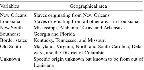
Table 1. Geographical regions in the sample
Variables Geographical area
New Orleans Slaves originating from New Orleans
Louisiana Slaves originating from all other areas in Louisiana New South Mississippi, Alabama, Texas, and Arkansas Southeast Georgia and Florida
Border states Kentucky, Tennessee, and Missouri
Old South Maryland, Virginia, North and South Carolina, Dela-ware, and the District of Columbia
Unknown Specific origin unknown but known to be from out of Louisiana
we lose a total of 547 observations due to incomplete infor-mation, leaving a final sample of 4,462 observations. In Sec-tion A.3 of the Data Appendix, we also provide summary sta-tistics comparing the deleted observations and the selected sam-ple. The histogram plots for prices and age suggest that there is no obvious systematic difference between the deleted and se-lected observations. We are reasonably confident that our data construction process is not systematically throwing away obser-vations of a particular type.
The selected 4,462 observations were classified into eight different regions based on the geographical origin of the slaves. They are New Orleans, Louisiana, New South, Old South, Bor-der states, and out of state, origin unknown. Table 1 gives the states for these regions and Figure 1 maps these states. For ease of the reader, a few tables are within the text, but the remainder are attached at the end of the article.
As a check of our sample, we compare a price deflator de-rived as the mean price for a male field hand slave between the ages of 21 and 35 with that derived by Ulrich B. Phillips (1929). This age interval is the same as that used by Kotlikoff (1979) and Fogel and Engerman (1974a). A comparison of the
de-Figure 1. Geographical origins of slaves.
Figure 2. Comparing Phillips’ price index with the indices derived from our sample.
rived price deflator and the commonly cited deflator by Phillips (1929) is given in Figure 2. The derived deflator appears to be more volatile than the Phillips series. The Phillips series also exceeds the derived deflator for part of the sample, most notably for the years between 1827 and 1832. However, the two series are highly correlated with a correlation coefficient of .82. The two series suggest a depression in slave prices occurring in the 1820s and in the 1840s. The latter coincided with a depression
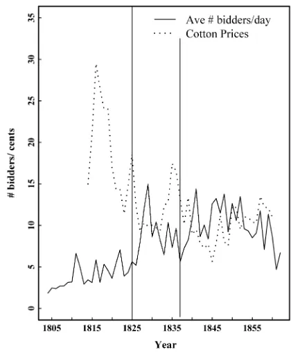
Figure 3. Average number of bidders/day and cotton price (in cents).
in cotton prices (also shown in Fig. 3). After around 1845, we observe an upward trend in the prices of slaves which continues until the pre-Civil War years of the 1860s. This increase coin-cides with a boom in the export market for cotton, as shown in Figure 4. (Data are taken from North 1966.) For most of the pe-riod considered, the derived deflator seems comparable to the Phillips series, suggesting that our sample is representative of the slave population over this period.
(a) (b)
Figure 4. (a) Volume of total exports and cotton exports (in millions of dollars). (b) Public land sales in five southern (ALA., ARK., LA., MISS., FLA.) (in millions of dollars). Note the scales on the left and right axes.
Table 2. Distribution of primary slaves by geographical origin and gender
Region No. of obs. Males Females
New Orleans 2,469 55.33 1,132 25.37 1,337 29.96
Table 2 gives the distribution of male and female slaves by geographical origin of all slaves. More than 50% of the sales transactions involve slaves originating from New Orleans, whereas only 13% came from the Old South. The remaining five regions each account for less than 10% of the total sales transactions. Table 3 provides a more detailed description of the data. Looking at the cumulative age profile, it appears that the majority of sales involve individuals aged 30 years and be-low. Around 40% of the sample are below 20 years old and another 40% are between the ages of 20 and 30 years. Given that slavery was closely connected with agriculture, this con-centration in age groups where the individual is in his or her physical prime is not surprising. Around 87% of the sample are guaranteed; that is, the seller ensures that the individual slave
Table 3. Some descriptive statistics on the final sample in percentages
I) Age Distribution of Principal Slaves
Age categories % Males % Females
Age<10 years old 2.11 1.84
II) Distribution by Skills and Time of Transactions (in Percents)
Sales transactions in Q1 35.10 Field hands 87.76 Sales transactions in Q2 31.16 Artisans 1.41 Sales transactions in Q3 15.00 House workers 5.00 Sales transactions in Q4 18.74 Other skills 5.83
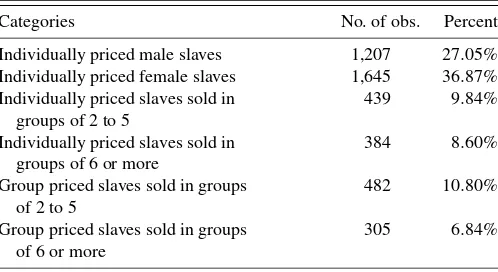
III) Distribution of Individually and Group Priced Slaves
Categories No. of obs. Percent
Individually priced male slaves 1,207 27.05% Individually priced female slaves 1,645 36.87% Individually priced slaves sold in
Group priced slaves sold in groups of 2 to 5
482 10.80%
Group priced slaves sold in groups of 6 or more
305 6.84%
is physically healthy. When a slave is not guaranteed, it is often because the individual was physically challenged or afflicted by an ailment which affected his or her ability to work. We find later that this status greatly affects individual sales prices.
The proportion that boasts specific specialized skills such as artisans and house-centered skills is small, totaling less than 10%. Artisan slaves are considered those slaves that acquired the following skills: Sail-maker, Blacksmith, Carpenter, Cabi-net maker, Cooper, Bricklayer, Mason, Butcher, Slater, Engi-neer, Tailor, and Shoe maker. House workers are those slaves with the following occupations: Gardener, Seamstress, House servant, Waiter, Domestic, Carriage driver, Hair dresser, Child nurse, and Baker. The majority of slaves in the sample are field hands. We observe that 60% of the slaves were sold in the first two quarters of the year whereas only 15% of sales actually oc-curred in the third quarter. This is something that we control for in our estimation. Around a third of the slaves (36%) are sold as part of a group, with half of these with a single group price. We also find that more females were sold individually than males (35% versus 27%). The majority of group sales involve groups of two to five individuals. Sales involving large groups of more than 10 individuals comprise around 10% of the sample. The proportion of sales involving children, that is, a child of age 10 or less, is small. Louisiana state law also prohibited the impor-tation of a child of less than 10 years of age without the child’s mother.
5.2 Aggregation
Group sales with a single price on the invoice are aggregated to yield an average price for the vector of average characteris-tics of slaves on the invoice whereas group sales with individu-ally listed prices are left as is. This aggregation leaves us with a final sample with 3,896 observations. Of these, 222 observa-tions are of aggregated group sales, and 214 observaobserva-tions are of single priced group sales. These amounted to 823 observations. The rest of the data are individually priced slaves. Of the indi-vidually priced slaves, males accounted for 1,207 observations and females accounted for the other 1,644 observations (see Ta-ble 2). Of the individually priced females, 336 were sold with accompanying children. None of the males had children accom-panying them. This aggregation of group sales introduces group heterogeneity that is captured by the termh(Zℓ)in the estimat-ing equation (2). This is one dimension by which we differ from Greenwald and Glasspiegel (1983) and Pritchett and Chamber-lain (1993), who ignored observations involving group sales. In addition to the group heteroscedasticity, we also account for time heteroscedasticity by including year and month fixed ef-fects.
5.3 Slave Hire Data
The slave sales data described above do not contain informa-tion on the number of bidders. As a consequence, we estimate the number of bidders participating in an auction using informa-tion from the slave sales data and an alternate slave hire dataset. The demand for slaves is driven by the need for labor inputs in agriculture. At any period in the sample, we assume that de-manders of slave labor could either purchase slaves from a sec-ondary slave market like New Orleans, or hire slaves from slave
owners. In other words, the pool of individuals who either pur-chased slaves or hired slaves implicitly defines the number of bidders participating in the New Orleans market. Using infor-mation about hiring transactions over the period of the sample, we construct an estimate of this quantity.
The slave hire data that we use can also be obtained from ICPSR (7422) at the University of Michigan. These data were obtained from a nonrandom sample of probate records for southern counties, located on microfilm at the Genealogical So-ciety Library of the Church of Jesus Christ of Latter Day Saints in Salt Lake City, Utah. These annual data contain the records of 20,253 slave hires in the south between 1775 and 1865. The data contain information on the year of the transactions, key identifiers for states as well as counties, and variables describ-ing the slave hired as well as the conditions of the hirdescrib-ing itself. We combine the annual hiring transactions with the monthly to-tal auction sales to construct a proxy of the number of bidders for each month for which we have sales transaction data. We are implicitly assuming that the number of bidders is on aver-age the same across auctions for each month of the sample. We feel that this approximation is not unreasonable. There is also evidence that the mean length of time it took a seller to sell a slave in New Orleans was about 40 days; see Freudenberger and Pritchett (1991).
Let mty be the weighted number of sales transactions in
month t in year y, where y=1804, . . . ,1862. The sampling weights for the sales data are either 2.5% or 5%. These weights are not arbitrarily chosen but are defined by Fogel and Engel-man who collected the data.hyis the number of hiring
transac-tions in yeary. The daily estimate of the number of bidders for all auctions in monthtof yearyis given by
nty=
In words, our estimate of the number of bidders is equal to the sum of the number of sales transactions and the number of hiring transactions weighted by the relative proportion of sales transactions for that month, divided by 30 days. Given that we have no prior on how hiring transactions are distributed over the months of the year, we thought using relative weight defined by sales fluctuations was a reasonable approximation.
Figure 3 also graphs the estimated average number of bid-ders per day participating in the New Orleans auctions and the price of cotton from this period. Our estimates suggest that the number of bidders more than doubled over our sample. At the beginning of the sample, around 1810, the average number of bidders participating in an auction was around 5, and this grew to around 10 by 1860. The estimated series shows two sharp in-creases over the sample period. The first, which began around 1825, appears to lag a sharp increase in cotton prices which be-gan in 1823. This also coincides with a sharp increase in the proportion of cotton exports to total exports in that same year as shown in Figure 4(a). The second major increase in the esti-mated bidders occurs in the late 1830s. Like the earlier increase, this seems to follow closely the 1835 boom in the cotton indus-try (prices and exports). Another significant event that explains this increase in demand for slaves is the expansion of agricul-tural land as reflected by the big increase in public land sales in this region around 1835. This is shown in Figure 4(b) which
plots the revenue from public land sales in five southern states measured in millions of dollars. The five states are Alabama, Arkansas, Mississippi, Louisiana, and Florida. The period be-tween 1814 and 1960 saw enormous growth in the demand for cotton from the British textile industry. (See Engerman, Sutch, and Wright 2004.) Despite this increase in demand, the gen-eral downward trend in cotton prices from 1814 to 1860 reflects the massive increase in supply brought about by the opening of new lands for cotton and the great westward migration over this period. North (1966) provided an excellent discussion of these events. These series, taken from North (1966), provide a gauge of whether the constructed series are a reasonable reflection of demand for slaves over this period. In general, the evidence in Figures 2, 3, and 4 suggests that the constructed series provide a reasonable approximation of the demand for slaves over this period.
6. RESULTS
The sample is a repeated cross section with varying numbers of observations for each month from 1804 to 1862. One would expect the price of slaves to fluctuate over this period according to the economic forces of supply and demand of the cotton tex-tile industry, and the sociopolitical climate of that time. These changes in demand (which are unobserved to the econometri-cian) affect the price of all slaves and could potentially be cor-related with any regional variations in slave prices. We need to control for these price fluctuations to ensure that any identified regional variation is not directly caused by demand changes. The inclusion of the number of bidders controls for the compet-itive environment at the time of the auction. We consider two approaches to control for unobserved demand conditions. The first deflates each price by a price index that would account for any economy-wide change in demand. The second accounts for these demand shifts using year, month, and year-month interac-tion dummy variables.
Equation (E1) below gives the empirical specification of our model (3) where we account for demand fluctuations using time dummy variables. This specification generates a string of coef-ficients for each year and month. A baseline specification of this model where we omit the effect of the number of bidders on the winning price is given by (E1b).
As discussed in Section 5, we construct a reliable deflator using the average price for individually priced, male field hand slaves between the ages of 21 and 38. These criteria allow us to construct a reasonably homogeneous subsample with which to construct the price deflator. Equation (E2) gives the empir-ical specification of our model (3) with deflated prices as the dependent variable and (E2b) gives the corresponding baseline regression [where we omitf(nℓ,t)].
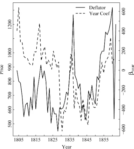
A time series plot of the derived deflator and the dummy vari-able coefficient estimates from the first approach are shown in Figure 5. We observe that after accounting for an interaction of year and month effects, the deflator index and the year coeffi-cient estimates trend in the same direction. Both series showed a depression in slave prices in the 1820s and the 1840s. The results from both approaches are found to be very similar:
Pℓt=XℓtβX+RℓtβR+SℓtβS+h(Zℓt)·f(nℓt)+ξℓt, (E1)
Pℓt=XℓtβX+RℓtβR+SℓtβS+ξℓt, (E1b)
Figure 5. Comparing the price deflatordt and year-month
coeffi-cientβyear.
Pℓt/dt=XℓtβX+RℓtβR+h(Zℓt)·f(nℓt)+ξℓt, (E2)
Pℓt/dt=XℓtβX+RℓtβR+ξℓt. (E2b)
The variables in these equations are:
Pℓtis the winning bid on auctionℓatt,
Rℓtare the regional dummy variables with coefficientsβR,
Sℓt includes year and year interacted with month dummy
variables; its coefficients are denoted byβT,
Xℓt are the remaining characteristics of the slave (other
than age and geographical origin) which also include the month when the slave is on auction,
nℓtis the estimated number of bidders participating in this
auction with the nonparametric effect captured byf(nℓt),
h(Zℓ)is a matrix with the reciprocal of the “lot” size on the diagonal and zero elsewhere (to control for group het-erogeneity),
dtis our derived price deflator for timetof the auction.
Table 9 defines the covariates used. We use Robinson’s (1988) double residual method to estimate theβ’s. Previous au-thors such as Greenwald and Glasspiegel (1983) and Pritchett and Chamberlain (1993) claimed that there was a significant structural change in the market for slaves before 1830 and af-ter. A number of incidents may have had a significant effect and have contributed to this structural change. For example, the first railroad which ran from the Elysian fields to Milnburg was built in 1830. This would have had a significant effect on transporta-tion costs; see Martin (1975, p. 13). New Orleans also had a cholera epidemic outbreak in 1831 which made it riskier to go to New Orleans. The cholera epidemic killed 6,000 people in just 20 days in New Orleans; see Martin (1975, pp. 13–14). The 1830s also brought major changes in legislation governing the importation of slaves from outside of Louisiana. As a result of dishonest trading behavior of selling “undesirable” or problem-atic slaves as prime slaves, the Louisiana legislature passed an
act in April 1829 which required a certification of good char-acter for all imported slaves. As a robustness check, we also consider a specification that allows for this structural change in the coefficient estimates in 1830. Our numerous tests for struc-tural break confirm that these changes in the 1830s had a sig-nificant effect on the parameter estimates. Some of the results of these specification tests have been put in Section A.2 of the Appendix.
We eventually arrive at the specifications in (E3) and (E4) be-low, which allow for the coefficient of the age polynomials and regional dummies to be different for the period before and after 1830. We also consider the baseline model where we omit the correction term accounting for the number of bidders in (E3b) and (E4b):
Pℓt=(1−I30)[XℓtβX+RℓtβR] +I30[XℓtβX30+RℓtβR30]
+SℓtβS+h(Zℓt)·f(nℓt)+ǫℓt, (E3)
Pℓt=(1−I30)[XℓtβX+RℓtβR] +I30[XℓtβX30+RℓtβR30]
+SℓtβS+ǫℓt, (E3b)
Pℓt/dt=(1−I30)[XℓtβX+RℓtβR] +I30[XℓtβX30+RℓtβR30]
+h(Zℓt)·f(nℓt)+ǫℓt, (E4)
Pℓt/dt=(1−I30)[XℓtβX+RℓtβR] +I30[XℓtβX30+RℓtβR30]
+ǫℓt. (E4b)
In (E3) and (E3b), we use year and month fixed effects to account for demand fluctuations, whereas in (E4) and (E4b), we use our constructed price deflator. In our test of the coeffi-cient of the remaining covariates, we fail to reject the null that the coefficients over these two periods are equal. The indicator variableI30 takes the value 1 for the period 1830 to 1862 and zero otherwise.
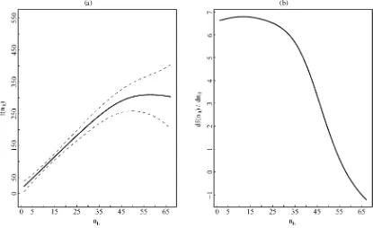
Our semiparametric estimation methodology allows us to identify the effect of the number of bidders on the winning price of slaves up to an additive constant. Figures 6(a) and 7(a) graph the nonparametric estimate of the number of bidders,f(nℓt), for
the specification in (E1) and (E3) together with the standard er-ror bands for these estimates. These standard erer-ror bands are pointwise 95% confidence intervals for our estimates off(nℓ). Figures 6(b) and 7(b) graph the marginal effect of the number of bidders on the average price of slaves on auction computed by numerically differentiating our estimates off(nℓt). Recall that
the dependent variable in both these specifications isPℓt. The
shape off(nℓt)and its corresponding derivatives for
specifica-tions (E2) and (E4) are very similar. Our estimates from both specifications suggest that the number of bidders has a signifi-cant positive effect on the average winning bid. For example, all else equal, the estimates from (E3) suggest that increasing the number of bidders from 20 to 30 would raise the average price of an individually priced slave by around $73. The predicted av-erage prices from specification (E1) for male and female field hands (evaluated at their respective averages) are around $692 and $606, respectively. So the competitive effect from increas-ing the number of bidders by 10 would raise the average prices for male and female field hands by around 10% and 12%, re-spectively.
(a) (b)
Figure 6. Estimates off(nℓt)and df(nℓ,t)/dnℓ,t for (E1). (a) Nonparametric estimate off(nlt)with standard error bands. (b) Numerical
estimate ofdf(nlt)/dntl.
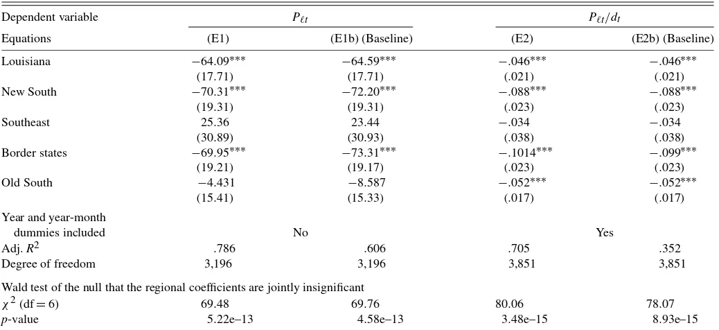
Table 4 gives the estimates for the regional coefficients for specifications (E1) and (E2) and their corresponding base re-gression described earlier. The omitted regional dummy vari-able is that of New Orleans. The estimates involving structural change from (E3) and (E4) are tabulated in Table 5. The esti-mates of the remaining covariates are in Tables 10–12 of the Appendix. Although the estimated coefficients of the model are
quantitatively different, the qualitative interpretation for all four specifications are similar.
Focusing on the estimate of (E3) in Table 5, the estimates pre-1830 suggest that slaves originating from “Old South,” “Border States,” and “New South” were discounted relative to slaves from “New Orleans.” Slaves from the “Border States” like Ken-tucky, Tennessee, and Missouri are the most heavily discounted,
(a) (b)
Figure 7. Estimates off(nℓt)and df(nℓ,t)/dnℓ,t for (E3). (a) Nonparametric estimate off(nlt)with standard error bands. (b) Numerical
estimate ofdf(nlt)/dntl.
Table 4. Regional coefficients from double residual regression of (E1) and (E2)
Dependent variable Pℓt Pℓt/dt
Equations (E1) (E1b) (Baseline) (E2) (E2b) (Baseline)
Louisiana −64.09∗∗∗ −64.59∗∗∗ −.046∗∗∗ −.046∗∗∗ (17.71) (17.71) (.021) (.021) New South −70.31∗∗∗ −72.20∗∗∗ −.088∗∗∗ −.088∗∗∗
(19.31) (19.31) (.023) (.023)
Southeast 25.36 23.44 −.034 −.034
(30.89) (30.93) (.038) (.038) Border states −69.95∗∗∗ −73.31∗∗∗ −.1014∗∗∗ −.099∗∗∗
(19.21) (19.17) (.023) (.023)
Old South −4.431 −8.587 −.052∗∗∗ −.052∗∗∗
(15.41) (15.33) (.017) (.017) Year and year-month
dummies included No Yes
Adj.R2 .786 .606 .705 .352
Degree of freedom 3,196 3,196 3,851 3,851
Wald test of the null that the regional coefficients are jointly insignificant
χ2(df=6) 69.48 69.76 80.06 78.07
p-value 5.22e–13 4.58e–13 3.48e–15 8.93e–15
NOTE: Significance codes: ***: 1%, **: 5%, *: 10%; month fixed effects are included in all specifications, no. of observations=3,896.
Table 5. Regional coefficients from double residual regression of (E3) and (E4)
Pℓt Pℓt/dt
Dependent variable (E3) (E3b) (Baseline) (E4) (E4b) (Baseline)
βR
Louisiana −27.28 −25.66 −.028 −.030
(27.72) (27.74) (.030) (.030) New South −119.4∗∗∗ −125.6∗∗∗ −.149∗∗∗ −.146∗∗∗
(38.33) (38.33) (.045) (.045)
Southeast −39.31 −37.35 −.111∗∗∗ −.111∗∗∗
(46.44) (46.50) (.055) (.055) Border States −130.5∗∗∗ −129.9∗∗∗ −.181∗∗∗ −.174∗∗∗
(30.74) (30.77) (.036) (.036) Old South −47.92∗∗∗ −50.67∗∗∗ −.066∗∗∗ −.064∗∗∗
(24.48) (24.49) (.027) (.027) βR30
Louisiana −94.53∗∗∗ −96.13∗∗∗ −.077∗∗∗ −.076∗∗∗ (22.75) (22.75) (.028) (.028) New South −51.54∗∗∗ −51.53∗∗∗ −.058∗∗∗ −.059∗∗∗
(22.02) (22.04) (.026) (.026)
Southeast 53.47 49.15 −.006 −.002
(40.89) (40.89) (.050) (.050) Border states −33.68 −40.64∗∗∗ −.065∗∗∗ −.063∗∗∗
(24.68) (24.61) (.029) (.029)
Old South 21.81 17.04 −.041∗∗∗ −.041∗∗∗
(19.62) (19.51) (.021) (.022) Year and year-month
dummies included No Yes
Adj.R2 .794 .619 .720 .384
Wald test of the null that the regional coefficients are jointly insignificant
χ2(df=12) 78.68 78.76 83.19 80.99
p-value 7.35e–12 7.12e–12 1.014e–12 2.67e–12
NOTE: Significance codes: ***: 1%, **: 5%, *: 10%, month and year-month fixed effects included in all specifications, no. of observations=3,896, degree of freedom=3,163.
followed by slaves from the “New South” and the “Old South.” All else equal, slaves from the “New South” were on average $70 cheaper relative to slaves from the “Old South.” Slaves originating from Louisiana (but outside of New Orleans) are not priced differently compared to slaves from New Orleans. When compared to the unconditional mean of singly priced slaves of $750, “New South” slaves were on average 9% cheaper relative to “Old South” slaves and almost 16% cheaper relative to slaves from New Orleans.
The post-1830 parameter estimates from (E3) suggest no sig-nificant price differential between slaves from the three regions of “Old South” and the “Border States” and those from “New Orleans.” However, slaves originating from the “New South” and Louisiana remain heavily discounted compared to slaves from New Orleans. The discount on Louisiana slaves increased whereas that on “New South” slaves decreased in this later pe-riod. After 1830, Louisiana slaves were the most heavily dis-counted, followed by slaves from the New South. When we omit the semiparametric correctionf(nℓ)in (E3b), we get some small changes in the magnitude of the parameter estimates. The qualitative results remain largely unchanged. The one notable difference is that the discount on “Border State” slaves post-1830 is now significant.
The qualitative results using deflated prices from (E4) are very similar to those from (E3). The main notable difference is that pre-1830, there is a systematic discount on slaves orig-inating from all regions outside of Lousiana. This includes the “Southeast” regions which include states like Georgia and Florida. In specification (E3), slaves from the “Southeast” earned a premium statistically similar to slaves from New Or-leans. Slaves from the “Border States” remain the most heav-ily discounted, followed by those from the “New South,” the “Southeast,” and the “Old South.” Post-1830, there are no sig-nificant discounts on slaves originating from the “Southeast” whereas there is a small discount on Louisiana slaves.
The estimates from (E1) and (E2) in Table 4 tell a very sim-ilar story of discounting on slaves from “Louisiana,” “Border States,” and “New South.” The general pattern of regional dis-counts is similar to the results of (E3) and (E4). In (E1), the estimates suggest that slaves from the “Old South” are not sys-tematically different in price from slaves from New Orleans. Nonetheless, slaves from the “Old South” still on average earn a $65 premium relative to slaves originating from the “New South.”
One result that seems robust in all of the specified models is that slaves originating from New Orleans on average com-manded a premium relative to slaves from other regions. This result is new to this literature and was not noted in earlier stud-ies. This positive premium could reflect the lower risk associ-ated with local slaves or an informational advantage of a local seller’s reputation. Comparing “New South,” “Border States,” and “New Orleans” regions, we also find strong evidence of a negative premium paid on slaves from “New South” and “Bor-der States,” with the latter on average more heavily discounted. There is some anecdotal evidence alluding to the high risk as-sociated with slaves imported from the “New South” and the “Border States.” We also find some evidence that slaves from the “Old South” receive a premium relative to slaves from the “New South.” This result confirms the findings of earlier work
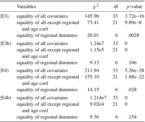
Table 6. Wald tests for structural break
Variables χ2 df p-value
(E3) equality of all covariates 145.96 33 3.72e–16 equality of all except regional
and age coef
73.41 21 9.89e–8
equality of regional dummies 20.01 6 .0028 (E3b) equality of all covariates 1.24e7 33 0
equality of all except regional and age coef
1.15e5 21 0
equality of regional dummies 9.13 6 .166 (E4) equality of all covariates 211.94 33 5.26e–28
equality of all except regional and age coef
155.10 21 1.88e–22
equality of regional dummies 14.15 6 .028 (E4b) equality of all covariates 1.214e7 33 0
equality of all except regional and age coef
9.02e4 21 0
equality of regional dummies 9.36 6 .154
using these data. We will defer the discussion of possible expla-nations for these persistent regional price variations to the next section. The last two rows of Tables 4 and 5 also provide the Wald test statistics of the null that all the regional coefficients are equal to that of New Orleans. Theχ2test statistic strongly rejects the null in all specifications, confirming that there is sig-nificant regional price variation.
We also test for the equality of coefficients pre- and post-1830, that is, β−β1830=0. These tests are done for varying subsets of coefficients from specifications (E3) and (E4) and their corresponding base specifications. The results are given in Table 6. When we test for equality of the coefficients on all covariates over the two periods, we consistently reject the null. With one exception, in the base regressions (E3b) and (E4b) where we do not account for the omitted number of bidders, we find that we accept the null of equality of the regional dummy coefficients over the two periods. In other words, failing to ac-count for the competitive effects of the number of bidders will lead to the incorrect conclusion that the regional coefficients over the two periods are equal.
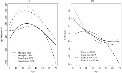
Figure 8(a) graphs the age polynomials of males and females for each of the periods implied by the estimates from (E3). Fig-ure 8(b) gives the partial derivative of the price of slaves with respect to age. We note that infant females were more valued than infant males (in both periods). However, this price differ-ential diminishes quickly with age. Male slaves age 9 and above (all else equal) on average received a higher price than female slaves. Interestingly enough, male prices outgrew female prices at the same age in the periods pre- and post-1830. The estimates on the remaining covariates are shown in Tables 10–12 of the Appendix. Reassuringly, these results conform to those of ear-lier work in this literature.
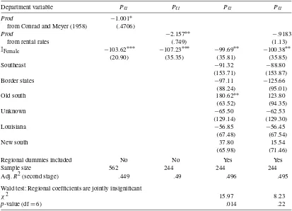
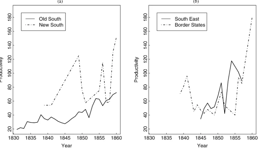
6.1 Explaining Regional Price Variation
Even after controlling for the competitive nature of the auc-tion market, significant price variaauc-tion across slaves’ geograph-ical origin continues to persist. This price differential between the “Old South” and the “New South” has been noted in earlier